The Linear Algebra Notes
Contents
- 0. Introduction
- 1. Vectors and Linear Combination
- 2. Matrices and Linear Transformation
- 3. Determinant
- 4. Equations, Inverse Matrices and Rank
- 5. Elimination with Matrices
- 6. Nonsquare Matrices, Dot Products, Cross Products and Solving System of Linear Equations
- 7. Cramer’s Rule
- 8. Change of Basis
- 9. Eigenvectors, Eigenvalues and Diagonalization
- 10. Abstract Vector Spaces
- 11. Graphs and Networks
- 12. Orthogonal Vectors and Matrices
- 13. Properties of Determinants
- 14. Difference Equations, Differential Equations (ODE) and exp(At)
- 15. Markov Matrices and Fourier Series
- 16. Complex Vectors, Complex Matrices and Fast Fourier Transform (FFT)
- 17. Symmetric Matrices and Positive Definiteness
- 18. Similar Matrices and Jordan Form
- 19. Singular Value Decomposition (SVD)
- 20. Left and Right Inverses; Pseudoinverse
- 98. Proofs of Some Properties
- 99. Terminologies in Different Languages
0. Introduction
This page is about the note of linear algebra. Myriads of students focus too much on the numeric concept of linear algebra, but the geometrical understanding is also worth considering. So here is a linear combination note combining the lecture by MIT-1806 and The essence of linear algebra by 3B1B.
If the formulae showed in this page are not displayed correctly, please try refreshing the page. The display of formulae bases on $\LaTeX$ and the render engine is MathJax.
If you want to jump to some chapter, it’s recommended to scroll the page to the end first, or the page may be scrolled back for the finishing of image loading after jumping.
To scroll the page to the end, you can click the last chapter or press the key (Ctrl+End) on the keyboard.
The contents are not arranged sequentially from the lectures mentioned above.
What should be noticed is that this is not a serious thesis or paper. In order to make the content more comprehensible, there may be not-strict-enough expressions and even mistakes.
If there is any fatal mistake exists, please leave a comment or send an e-mail to me.
Not all images in this page is original. Some of them come from the Internet.
This article is the new version, replacing the old one written in 2022.7.9.
1. Vectors and Linear Combination
1.1 What is the vector
Vector is the bedrock of linear algebra. But what the vector really is?
In mathematical concept, vector can be described as an arrow starts on an origin and points at one direction. The vector can be placed on anywhere, but we can fix it on the origin point of a coordinate system.
Imagine there is a 2-dimensional coordinate with two perpendicular x-axis and y-axis.
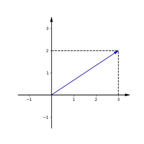
And we can describe this vector as $\mathbf{\hat v} = \begin{bmatrix} 3 \\ 2 \end{bmatrix}$. The numbers tell another point in the coordinate where the vector points at.
1.2 The addition and multiplication of vectors
If we and two vectors together, it means move the second vector’s tail to the tip of the first one, and where the tip of the second vector sits is the sum of two vector.
If we multiply a vector by a number, it scales the vector. If the multiplier number is negative, it reverses the vector.
The numbers used to scale the vector is called scaler.
$$
\begin{equation}
a \cdot
\begin{bmatrix} x \\ y \end{bmatrix}
=
\begin{bmatrix} a \cdot x \\ a \cdot y \end{bmatrix}
\end{equation}
$$
There are two special vectors $\hat i = \begin{bmatrix} 1 \\ 0 \end{bmatrix}$ and $\hat j = \begin{bmatrix} 0 \\ 1 \end{bmatrix}$, which are called unit vectors.
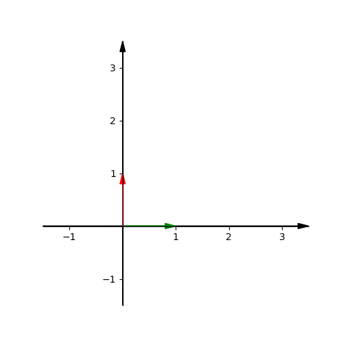
If we scale these two vectors and add them together, it produces a new vector. Whatever the new vector is, these must be a scaler $a$ and a scaler $b$ to produce it. That means if we draw all the vectors produced by the multiplication and addition of $\hat i$ and $\hat j$, it will fill all space in the plane. The $\hat i$ and $\hat j$ are the basis vectors of the xy coordinate.
When we scale two vectors and add them together, it’s called linear combination.
1.3 What if we can choose different basis vectors?
If we choose two random vectors and scale them and add them together, it can also produce a new vector. But if these two basis vectors are paralleled, that means two vectors are unfortunately in the same line, the new result vector will be limited in a line. If one of the original vectors is zero, the new result vector will be zero.
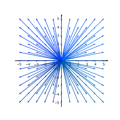
The set of all possible vectors that you can reach with a linear combination of a given pair of vectors is called the span of those two vectors.
So we can say, the span of most pairs of 2D vectors is all vectors of 2D space. But when they line up, the span is all vectors whose tip sit on a certain line.
If this pair of 2D vectors(not zero) $\vec u$ and $\vec v$ are line up, one of them can be scaled to produce another one. In this situation, $\vec u = a \vec v$. We say $\vec u$ and $\vec v$ are linearly dependent.
If two vectors are line up, the span has one dimension. If they are not, the span would be 2 dimensions.
In 3-dimensional space, the span of two vectors can only be a flat as possible. If we add the third vector, and when it is outside the flat of other two vectors, the span will be expanded to 3 dimensions. If each vector does add another dimension to the span, they are said to be linearly independent.
The basis of a vector space is a set of linearly independent vectors that span the full space.
2. Matrices and Linear Transformation
2.1 What is transformation
Linear transformation is like a function. It takes in inputs and produces outputs.
$$
inputs \rightarrow f(x) \rightarrow outputs
$$
In the context of linear algebra, it takes in vector and outputs another vector.
$$
\vec u \rightarrow L(\vec v) \rightarrow \vec w
$$
Imagine there is an image consists series of points, a transformation scales, rotates, and even distorts the image.
Fortunately linear transformation won’t curve a line, that’s why it is called linear.
In a linear transformation, the line will still be a line, and the origin will not move.
If a linear transformation applied with $\hat i$, $\hat j$ and $\vec v = a\hat i + b\hat j$, there will be $\hat i_{transformed}$, $\hat j_{transformed}$ and $\vec v_{transformed} = a\hat i_{transformed} + b\hat j_{transformed}$.
So if we transform $\hat i = \begin{bmatrix} \color{green}1 \\ \color{green}0 \end{bmatrix}$ to $\hat i_{transformed} = \begin{bmatrix} \color{green}3 \\ \color{green}-2 \end{bmatrix}$ and $\hat j = \begin{bmatrix} \color{red}0 \\ \color{red}1 \end{bmatrix}$ to $\hat j_{transformed} = \begin{bmatrix} \color{red}2 \\ \color{red}1 \end{bmatrix}$, then all the vectors produced by the two basis vectors can be easily transformed by multiplication and addition of the two basis vectors.
2.2 Matrix
The pack $\hat i_{transformed}$ and $\hat j_{transformed}$ into a 2x2 grid of numbers is called a 2x2 matrix.
$$
\begin{bmatrix}
\color{green}3 & \color{red}2 \\
\color{green}-2 & \color{red}1
\end{bmatrix}
$$
It tells where the two special basis vectors land after transformation. It also tells where the other vectors land after this transformation.
For example, $\vec v=\begin{bmatrix} \color{orange}5 \\ \color{orange}7 \end{bmatrix}$, applied with the matrix above, then
$$
\begin{equation}
\vec v_{transformed} =
\color{orange}{5} \color{black}
\begin{bmatrix}
\color{green}3 \\
\color{green}-2
\end{bmatrix} +
\color{orange}{7} \color{black}
\begin{bmatrix}
\color{red}2 \\
\color{red}1
\end{bmatrix}
\end{equation}
$$
In general cases, we put a matrix on the left of the vector to transform the vector.
$$
\begin{equation}
\begin{bmatrix}
\color{green}a & \color{red}b \\
\color{green}c & \color{red}d
\end{bmatrix}
\begin{bmatrix}
\color{orange}x \\
\color{orange}y
\end{bmatrix}
=
\color{red}{x} \color{black}
\begin{bmatrix}
\color{green}a \\
\color{green}c
\end{bmatrix} +
\color{red}{y} \color{black}
\begin{bmatrix}
\color{red}b \\
\color{red}d
\end{bmatrix} =
\begin{bmatrix}
\color{green}a\color{orange}x + \color{red}b\color{orange}y \\
\color{green}c\color{orange}x + \color{red}d\color{orange}y
\end{bmatrix}
\end{equation}
$$
For example, let’s see what happens to $
\begin{equation}
\begin{bmatrix} \color{green}3 & \color{red}1 \\ \color{green}1 & \color{red}2 \end{bmatrix}
\begin{bmatrix} \color{orange}-1 \\ \color{orange}2 \end{bmatrix} =
\begin{bmatrix} \color{orange}-1 \\ \color{orange}3 \end{bmatrix}
\end{equation}
$
See another example. If you want to rotate all of space 90 degrees counterclockwise, then $\hat i$ lands on $\begin{bmatrix} \color{green}0 \\ \color{green}1 \end{bmatrix}$ and $\hat j$ lands on $\begin{bmatrix} \color{red}-1 \\ \color{red}0 \end{bmatrix}$.
So the matrix which can do this transformation is $
\begin{bmatrix}
\color{green}0 & \color{red}-1 \\
\color{green}1 & \color{red}0
\end{bmatrix}
$
To rotate any vector 90 degrees counterclockwise, you just multiply it by this matrix.
2.3 Matrix multiplication
We may want to apply two transformations, for example, firstly rotate the plane 90 degrees counterclockwise and then apply a shear. This is called the composition of a rotation and a shear.
To do this, we multiply the vector by a rotation matrix, then multiply it by a shear. Remember, when we apply a transformation, we put the matrix on the left.
we can also multiply the vector by a composition vector.
$$
\color{pink}
\underbrace{
\begin{bmatrix}
1 & 1 \\
0 & 1
\end{bmatrix}
}_{Shear}
\color{black}\bigg(
\color{green}
\underbrace{
\begin{bmatrix}
0 & -1 \\
1 & 0
\end{bmatrix}
}_{Rotation}
\color{black}
\begin{bmatrix}
x \\
y
\end{bmatrix}
\color{black}\bigg)
=
\underbrace{
\begin{bmatrix}
1 & -1 \\
1 & 0
\end{bmatrix}
}_{Composition}
\begin{bmatrix}
x \\
y
\end{bmatrix}
$$
We call the new composition matrix is the product of the original two matrices.
$$
\color{pink}
\underbrace{
\begin{bmatrix}
1 & 1 \\
0 & 1
\end{bmatrix}
}_{Shear}
\color{green}
\underbrace{
\begin{bmatrix}
0 & -1 \\
1 & 0
\end{bmatrix}
}_{Rotation}
\color{black}
=
\underbrace{
\begin{bmatrix}
1 & -1 \\
1 & 0
\end{bmatrix}
}_{Composition}
$$
This is the multiplication of matrices. And its geometrical meaning is to apply one transformation then another.
Notice that we read the multiplication from right to left. It means we apply the transformation represented by the matrix on the right, then apply the transformation represented by the matrix on the left.
But if we change the sequence, to apply the shear first, then rotation. What will happen?
As you can see, in matrix multiplication, $AB \neq BA$.
How to calculate multiplication of matrices in numerical way? See this example:
$$
M_2M_1=
\begin{bmatrix}
0 & 2 \\
1 & 0
\end{bmatrix}
\begin{bmatrix}
1 & -2 \\
1 & 0
\end{bmatrix}
=
\begin{bmatrix}
\color{green}? & \color{red}? \\
\color{green}? & \color{red}?
\end{bmatrix}
$$
See the matrix $M_1$, it transforms $\hat i$ to $\hat i_{transformed}=\begin{bmatrix} 1 \\ 1 \end{bmatrix}$ and $\hat j$ to $\hat j_{transformed}=\begin{bmatrix} -2 \\ 0 \end{bmatrix}$.
Then $M_2$ catches up to transform the $\hat i_{transformed}$:
$$
\begin{bmatrix}
0 & 2 \\
1 & 0
\end{bmatrix}
\begin{bmatrix}
1 \\
1
\end{bmatrix}
=
\begin{bmatrix}
\color{green}2 \\
\color{green}1
\end{bmatrix}
$$
And $\hat j_{transformed}$ is also be transformed by $M_2$:
$$
\begin{bmatrix}
0 & 2 \\
1 & 0
\end{bmatrix}
\begin{bmatrix}
-2 \\
0
\end{bmatrix}
=
\begin{bmatrix}
\color{red}0 \\
\color{red}-2
\end{bmatrix}
$$
Then the composition matrix is the result combining two new vectors
$$
M_2M_1=
\begin{bmatrix}
0 & 2 \\
1 & 0
\end{bmatrix}
\begin{bmatrix}
1 & -2 \\
1 & 0
\end{bmatrix}
=
\begin{bmatrix}
\color{green}2 & \color{red}0 \\
\color{green}1 & \color{red}-2
\end{bmatrix}
$$
As you can see, the basis vectors are transformed twice then become new vectors. Then the new vectors are combined to be a new matrix telling the transformation represented by the combination of two matrices.
2.4 When are A and B allowed to be multiplied
The $m \times n$ matrix is signified as $M_{m \times n}$
We use $a_{ij}$ to describe the entry of $A$ on line i, column j.
$$
A_{\color{blue}{m}\times\color{red}{k}}
B_{\color{red}{k}\times\color{green}{n}}=
C_{\color{blue}{m}\times\color{green}{n}}
$$
That means the multiplication must be a left matrix with k columns and a right matrix with k rows.
If the left matrix has m rows, and the right matrix has n columns, the result will have m rows and n columns.
2.5 Five ways to calculate the multiplication of matrices.
2.5.1 Dot production of vector [$row_i$] and vector [$colomn_j$]
$$
\begin{bmatrix}
& & & \vdots \\
a_{i1} & a_{i2} & \cdots & a_{ik} \\
& & & \vdots
\end{bmatrix}
\begin{bmatrix}
& b_{1j} & \\
& b_{2j} & \\
& \vdots & \\
\cdots & b_{kj} & \cdots
\end{bmatrix}=
\begin{bmatrix}
& \vdots & & \\
\cdots & c_{ij} & \cdots & \\
& \vdots & &
\end{bmatrix}
$$
$$
c_{ij}=
\begin{bmatrix}a_{i1} & a_{i2} & \cdots & a_{ik}\end{bmatrix} \cdot
\begin{bmatrix}b_{1j}\\b_{2j}\\\vdots\\b_{kj}\end{bmatrix}
=a_{i1}b_{1j}+a_{i2}b_{2j}+\cdots+a_{ik}b_{kj}
=\sum^{k}_{p=1}a_{ip}b_{pj}
$$
2.5.2 Each column of C is the linear combination of A
$$
\begin{bmatrix}
A_{col_1} & A_{col_2} & \cdots & A_{col_k}
\end{bmatrix}
\begin{bmatrix}
\cdots & b_{1j} & \cdots \\
\cdots & b_{2j} & \cdots \\
\cdots & \vdots & \cdots \\
\cdots & b_{kj} & \cdots
\end{bmatrix}=
\begin{bmatrix}
\cdots & (b_{1j}A_{col_1} & b_{2j}A_{col_2} & \cdots & b_{kj}A_{col_k}) & \cdots
\end{bmatrix}
$$
2.5.3 Each row of C is the linear combination of B
$$
\begin{bmatrix}
\vdots & \vdots & \vdots & \vdots \\
a_{i1} & a_{i2} & \cdots & a_{ik} \\
\vdots & \vdots & \vdots & \vdots
\end{bmatrix}
\begin{bmatrix}
B_{row_1} \\ B_{row_2} \\ \vdots \\ B_{row_k}
\end{bmatrix}=
\begin{bmatrix}
\vdots \\
(a_{i1}B_{row_1} + a_{i2}B_{row_2} + \cdots + a_{ik}B_{row_k}) \\
\vdots \\
\end{bmatrix}
$$
2.5.4 Multiply columns of A by rows of B
$$
\begin{bmatrix}
A_{col_1} & A_{col_2} & \cdots & A_{col_k}
\end{bmatrix}
\begin{bmatrix}
B_{row_1} \\ B_{row_2} \\ \vdots \\ B_{row_k}
\end{bmatrix}=
A_{col_1}B_{row_1}+A_{col_2}B_{row_2}+\cdots+A_{col_k}B_{row_k}
$$
2.5.5 Block Multiplication
$$
\begin{bmatrix}\begin{array}{c | c}
A_1 & A_2 \\ \hline{} A_3 & A_4
\end{array}\end{bmatrix}
\begin{bmatrix}\begin{array}{c | c}
B_1 & B_2 \\ \hline{} B_3 & B_4
\end{array}\end{bmatrix}=
\begin{bmatrix}\begin{array}{c | c}
A_1B_1+A_2B_3 & A_1B_2+A_2B_4 \\ \hline{}
A_3B_1+A_4B_3 & A_3B_2+A_4B_4
\end{array}\end{bmatrix}
$$
2.6 Properties of Matrix Multiplication
- Commutative Law of Addition: $A+B=B+A$
- Associativity Law of Multiplication: $A(BC)=(AB)C$
- Left Distributive Law of Matrix Multiplication: $A(B+C)=AB+AC$
2.7 Other Basic Matrix Arithmetics And Terminologies
2.7.1 Identity Matrix
An identity matrix, sometimes called a unit matrix, is a diagonal matrix with all its diagonal entries equal to 1 , and zeroes everywhere else.
$$
I=
\begin{bmatrix}
1 & 0 & \cdots & 0 \\
0 & 1 & \cdots & 0 \\
\vdots & \vdots & \ddots & \vdots \\
0 & 0 & \cdots & 1
\end{bmatrix}
$$
After multiplying an identity matrix by a vector, it will do nothing to the vector.
2.7.2 Zero Matrix
A zero matrix is a matrix that has all its entries equal to zero.
$$
O=
\begin{bmatrix}
0 & 0 & \cdots & 0 \\
0 & 0 & \cdots & 0 \\
\vdots & \vdots & \ddots & \vdots \\
0 & 0 & \cdots & 0
\end{bmatrix}
$$
2.7.3 Diagonal Matrix
A zero matrix is a matrix whose entries are all zero except those in diagonal.
$$
D = diag(a_1,a_2,\cdots,a_n) =
\begin{bmatrix}
a_1 & 0 & \cdots & 0 \\
0 & a_2 & \cdots & 0 \\
\vdots & \vdots & \ddots & \vdots \\
0 & 0 & \cdots & a_n
\end{bmatrix}
$$
2.7.4 Addition and Subtraction
The sum (or difference) of two compatible matrices is a matrix of the same size, with each entry the sum (or difference) of the corresponding entries of the two matrices.
$$
\begin{bmatrix}
a_{11} & a_{12} & \cdots & a_{1n} \\
a_{21} & a_{22} & \cdots & a_{2n} \\
\vdots & \vdots & & \vdots \\
a_{m1} & a_{m2} & \cdots & a_{mn}
\end{bmatrix}
\pm
\begin{bmatrix}
b_{11} & b_{12} & \cdots & b_{1n} \\
b_{21} & b_{22} & \cdots & b_{2n} \\
\vdots & \vdots & & \vdots \\
b_{m1} & b_{m2} & \cdots & b_{mn}
\end{bmatrix}
=
\begin{bmatrix}
a_{11} \pm b_{11} & a_{12} \pm b_{12} & \cdots & a_{1n} \pm b_{1n} \\
a_{21} \pm b_{21} & a_{22} \pm b_{22} & \cdots & a_{2n} \pm b_{2n} \\
\vdots & \vdots & & \vdots \\
a_{m1} \pm b_{m1} & a_{m2} \pm b_{m2} & \cdots & a_{mn} \pm b_{mn}
\end{bmatrix}
$$
$$
c_{ij} = a_{ij} \pm b_{ij}
$$
2.7.5 Scalar
$$
\lambda A=
\lambda
\begin{bmatrix}
a_{11} & a_{12} & \cdots & a_{1n} \\
a_{21} & a_{22} & \cdots & a_{2n} \\
\vdots & \vdots & & \vdots \\
a_{m1} & a_{m2} & \cdots & a_{mn}
\end{bmatrix}
=
\begin{bmatrix}
\lambda a_{11} & \lambda a_{12} & \cdots & \lambda a_{1n} \\
\lambda a_{21} & \lambda a_{22} & \cdots & \lambda a_{2n} \\
\vdots & \vdots & & \vdots \\
\lambda a_{m1} & \lambda a_{m2} & \cdots & \lambda a_{mn}
\end{bmatrix}
$$
$$
-A=(-1)A=
-
\begin{bmatrix}
a_{11} & a_{12} & \cdots & a_{1n} \\
a_{21} & a_{22} & \cdots & a_{2n} \\
\vdots & \vdots & & \vdots \\
a_{m1} & a_{m2} & \cdots & a_{mn}
\end{bmatrix}
=
\begin{bmatrix}
-a_{11} & -a_{12} & \cdots & -a_{1n} \\
-a_{21} & -a_{22} & \cdots & -a_{2n} \\
\vdots & \vdots & & \vdots \\
-a_{m1} & -a_{m2} & \cdots & -a_{mn}
\end{bmatrix}
$$
Properties:
- Associativity Law: $k(lA)=(kl)A$
- Left Distributive Law: $(k+l)A=kA+kB, k(A+B)=kA+kB$
- if $kA=0$, then $k=0$ or $A=0$
- $k(AB)=(kA)B=A(kB)$
2.7.6 the 𝑘th power of 𝐴
For a square matrix $A$ and positive integer 𝑘, the 𝑘th power of $A$ is defined by multiplying this matrix by itself repeatedly.
$$
\begin{align}
& A^1=A \\
& A^2=AA \\
& A^k=\underbrace{AA \cdots A}_{k}, k \in N \\
& A^k=A^{k-1}A, k=2, 3, \cdots \\
& A^0=I
\end{align}
$$
Properties:
- $A^{k}A^{l}=A^{k+l}$
- $(A^k)^l=A^{kl}$
2.7.7 Transpose
Switch the rows and columns of the matrix, so that the first row becomes the first column, the second row becomes the second column, and so on.
$$
A=
\begin{bmatrix}
a_{11} & a_{12} & \cdots & a_{1n} \\
a_{21} & a_{22} & \cdots & a_{2n} \\
\vdots & \vdots & & \vdots \\
a_{m1} & a_{m2} & \cdots & a_{mn}
\end{bmatrix}
$$
$$
A^T=
\begin{bmatrix}
a_{11} & a_{21} & \cdots & a_{m1} \\
a_{12} & a_{22} & \cdots & a_{m2} \\
\vdots & \vdots & & \vdots \\
a_{1n} & a_{m2} & \cdots & a_{mn}
\end{bmatrix}
$$
Properties:
- $(A^T)^T=A$
- $(A+B)^T=A^T+B^T$
- $(kA^T)=kA^T$
- $(AB)^T=B^{T}A^{T}$
A symmetric matrix is a square matrix which is symmetric about its leading diagonal: $A=A^T$
On two sides of the diagonal line the entries are identical:
$$
\begin{bmatrix}
\color{red}a & \color{blue}x & \color{green}y \\
\color{blue}x & \color{red}b & \color{purple}z \\
\color{green}y & \color{purple}z & \color{red}c
\end{bmatrix}
$$
Properties of symmetric matrix:
- The sum and difference of two symmetric matrices is symmetric.
- This is not always true for the product: given symmetric matrices $A$ and $B$, then $AB$ is symmetric if and only if $A$ and $B$ commute, i.e. if $AB=BA$.
- For any integer $n$, $A^n$ is symmetric if $A$ is symmetric.
- Rank of a symmetric matrix $A$ is equal to the amount of non-zero eigenvalues of $A$.
- Given any non-square matrix A, then $AA^T$ is a symmetric matrix.
An antisymmetric (or skew-symmetric) matrix is a matrix $A$ when $A^T=-A$
Properties of antisymmetric matrix:
- If you add two antisymmetric matrices, the result is another antisymmetric matrix.
- If you multiply an antisymmetric matrix by a constant, the result is another antisymmetric matrix.
- All of the diagonal entries of an antisymmetric matrix are 0.
3. Determinant
3.1 What is determinant
When a linear transformation be applied, then space is stretched or squashed.
If there is an area applied with a linear transformation, how much is the area scaled?
To measure the factor by which the area of a given region increases or decreased, we can focus on the unit 1x1 square formed by $\hat i$ and $\hat j$.
For example: $\begin{bmatrix} 3 & 0 \\ 0 & 2 \end{bmatrix}$
![]()
As you can see, the area of 1x1 square was scaled to 3x2, i.e. 6.
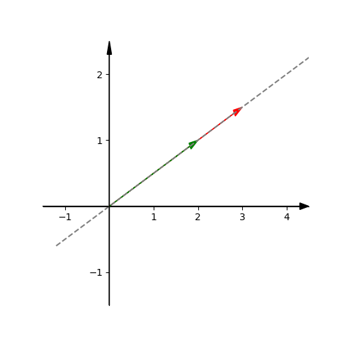
Another example: $\begin{bmatrix} 1 & 1 \\ 0 & 1 \end{bmatrix}$
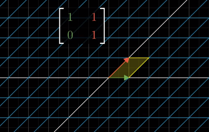
It’s easy to calculate that the area of this parallelogram is still 1 after transformation.
Actually, if you know how much the area of the unit square changes, it can tell you how the area of any possible region in space changes after transformation whatever the size is. Because the transformation is linear, as it’s noted before.
This very special scaling factor is called the determinant of the transformation.
$$
det(A)=det\bigg(
\begin{bmatrix}
a_{11} & a_{12} \\
a_{21} & a_{22}
\end{bmatrix}
\bigg)=
\begin{vmatrix}
a_{11} & a_{12} \\
a_{21} & a_{22}
\end{vmatrix}
$$
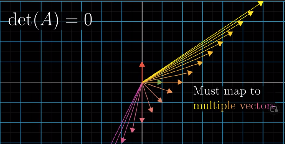
The value of the determinant tells the factor of the transformation. If the determinant is 0, it tells that all of the space are squished onto a line or even a single point. At this situation, the $\hat i_{transformed}$ and the $\hat j_{transformed}$ are linear dependent.
3.2 The sign of the determinant
But what if the determinant is negative? What’s the meaning of scaling an area by a negative number?
The sign of a determinant is all about orientation. If the determinant is negative, the transformation is like flipping the space over, or inverting the orientation of space.
Another way to think about it is that in the beginning $\hat j$ is to the left of $\hat i$. If after the transformation, $\hat j$ is on the right of $\hat i$, the orientation of space has been inverted, and the determinant will be negative.
3.3 Determinant of 3D linear transformation
In comparison with 2D, it’s about scaling volumes in 3D linear transformation.
After transformation, the unit 1x1x1 cube will be a parallelepiped, a plane, a line or a point.
the determinant of 3D linear transformation is the scaling factor of volumes, but what’s the meaning of the sign, or how to describe the orientation?
Right-hand rule:
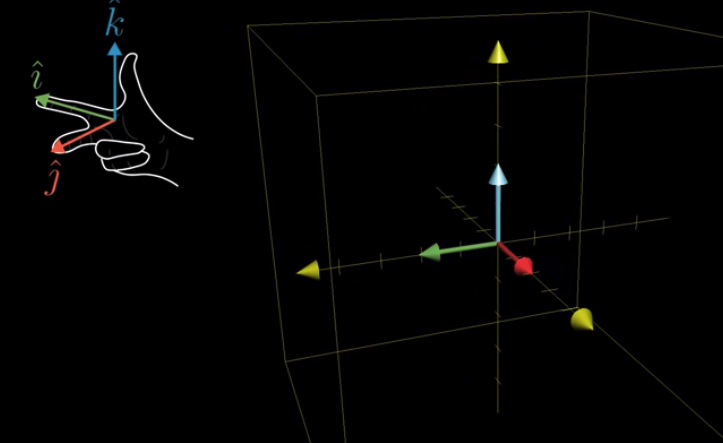
The image tells the orientation of positive determinant. Otherwise, it is negative.
3.4 How to calculate the determinant
In 2x2 case
$$
\begin{equation}
\begin{vmatrix}
\color{green}a & \color{red}b \\
\color{green}c & \color{red}d
\end{vmatrix}
=
\color{green}a \color{red}d - \color{red}b \color{green}c
\end{equation}
$$
It’s easy to prove: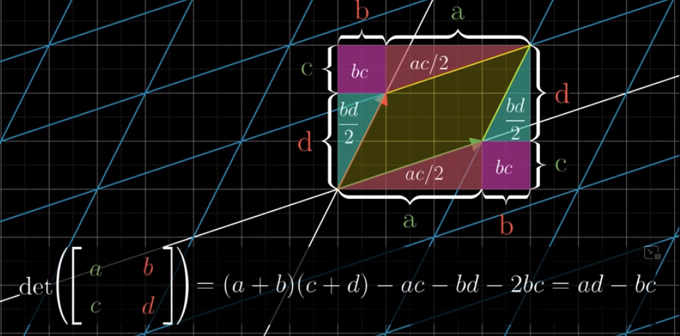
In 3x3 case
$$
\begin{equation}
\begin{vmatrix}
\color{green}a & \color{red}b & \color{blue}c \\
\color{green}d & \color{red}e & \color{blue}f \\
\color{green}g & \color{red}h & \color{blue}i
\end{vmatrix}
=
\color{green}a \color{black}
\begin{vmatrix}
\color{red}e & \color{blue}f \\
\color{red}h & \color{blue}i
\end{vmatrix}-
\color{red}b \color{black}
\begin{vmatrix}
\color{green}d & \color{blue}f \\
\color{green}g & \color{blue}i
\end{vmatrix}+
\color{blue}c \color{black}
\begin{vmatrix}
\color{green}d & \color{red}e \\
\color{green}g & \color{red}h
\end{vmatrix}
=
\color{green}a \color{red}e \color{blue}i \color{black}+ \color{red}b \color{blue}f \color{green}g \color{black}+ \color{blue}c \color{green}d \color{red}h \color{black}-
\color{green}a \color{blue}f \color{red}h \color{black}- \color{red}b \color{green}d \color{blue}i \color{black}- \color{blue}c \color{red}e \color{green}g
\end{equation}
$$
The details and tricks to calculate the determinant will be introduced in the ensuing chapters.
4. Equations, Inverse Matrices and Rank
4.1 A simple example of two equations with two unknowns
Linear algebra is useful in computer science, robotics and so forth. But one of the main reasons why linear algebra is broadly applicable is that it lets us solve certain systems of equations. And luckily this kind of equations are linear equations, which means the equations only consist of additions of unknowns scaled by some constant. No exponents or fancy functions or multiplying two variables together.
These do not exist in linear equations: $x^2$, $\sin x$, $xy$
$$
\begin{cases}
\ 2x&-y&=0 \\ -x&+2y&=3
\end{cases}
$$
And as you can see, all the unknowns vertically line up on the left and the lingering constants are on the right.
And you can package all of the equations together into a single vector equation like this:
$$
\begin{equation}
\underbrace{\begin{bmatrix} 2 & -1 \\ -1 & 2 \end{bmatrix}}_{A}
\underbrace{\begin{bmatrix} x \\ y \end{bmatrix}}_{\vec X}
=
\underbrace{\begin{bmatrix} 0 \\ 3 \end{bmatrix}}_{\vec b}
\end{equation}
$$
$A$ is coefficient matrix. $\vec X$ is vector of unknowns. $\vec b$ is vector of the right-hand numbers of equations.
Using three letters to express this three matrices:
$$ A\mathbf{X}=\mathbf{b} $$
That means we should look for a vector $\vec X$, which, after applying the transformation, lands on $\vec b$.
We can draw the row pictures of equations on a xy plane. Obviously They are two lines. all the points in each line are solutions of each equation.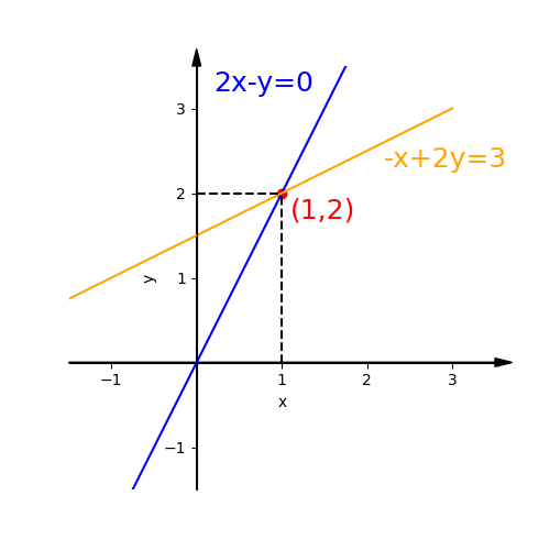
The intersection of two line is the solution of the equations.
Then the column pictures:
Focusing on the columns of matrix, we can get this:
$$
\begin{equation}
x \begin{bmatrix} 2 \\ -1 \end{bmatrix} + y
\begin{bmatrix} -1 \\ 2 \end{bmatrix} =
\begin{bmatrix} 0 \\ 3 \end{bmatrix}
\end{equation}
$$
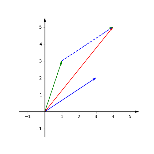
This equation is asking us to find the x and y to combine the vector $x\begin{bmatrix} 2 \\ -1 \end{bmatrix}$ and the vector $y\begin{bmatrix} -1 \\ 2 \end{bmatrix}$ to get the vector $\begin{bmatrix} 0 \\ 3 \end{bmatrix}$. That is the linear combination we need to find out.
Draw three vectors mentioned above. We already know the right x and y. So we can get the red vector when combining 2 green vectors and 1 blue vector.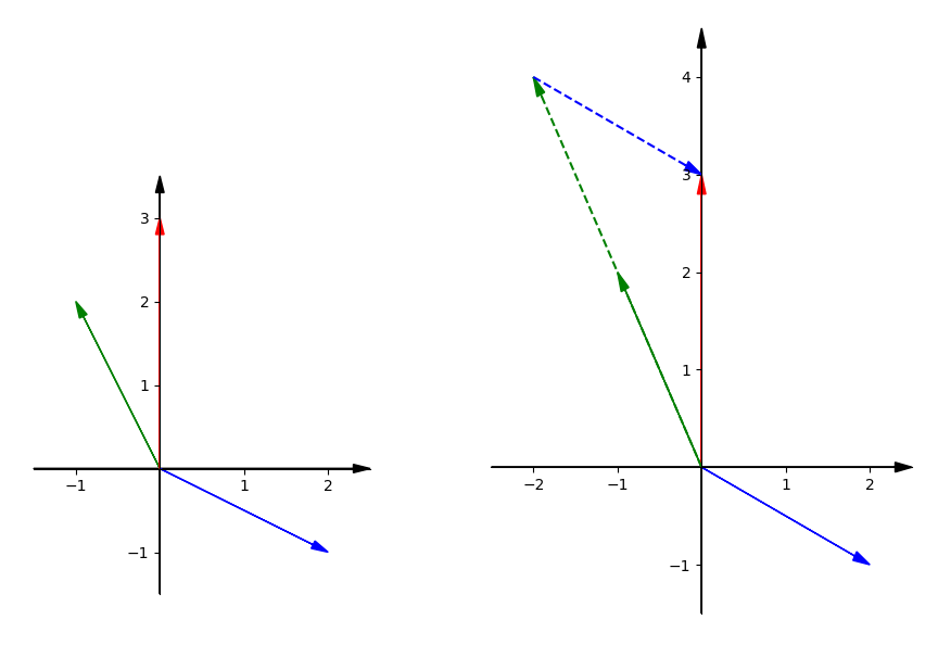
4.2 Three equations with 3 unknowns
\begin{cases}
2x & -y & &= 0 \\
-x & +2y & -z &= -1 \\
& -3y & +4z &= 4
\end{cases}
We can insert zero coefficients when the unknown doesn’t show up.
$$
\begin{cases}
2\color{green}x & \color{black}-1\color{red}y & \color{black}+0\color{blue}z\color{black} & =0 \\
(-1)\color{green}x & \color{black}+2\color{red}y & \color{black}-1\color{blue}z\color{black} & =-1 \\
1\color{green}x & \color{black}-3\color{red}y & \color{black}+4\color{blue}z\color{black} & =4
\end{cases}
$$
Package all of the equations together into a single vector equation like this:
$$
\begin{equation}
\underbrace{
\begin{bmatrix}
2 & -1 & 0 \\
-1 & 2 & -1 \\
0 & -3 & 4
\end{bmatrix}
}_{A}
\underbrace{
\begin{bmatrix}
\color{green}x \\
\color{red}y \\
\color{blue}z
\end{bmatrix}
}_{\vec X}
=
\underbrace{
\begin{bmatrix}
0 \\
-1 \\
4
\end{bmatrix}
}_{\vec b}
\end{equation}
$$
See the row pictures:
Firstly draw two planes(2x-y=0 and -x+2y-z=-1). These planes meet in a line.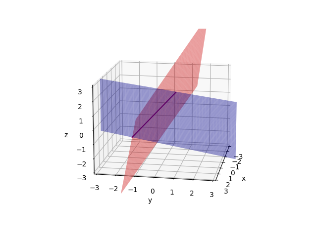
Then draw the third plane(-3y+4z=4).They meet in a point(0, 0, 1). And this point is solution of equations.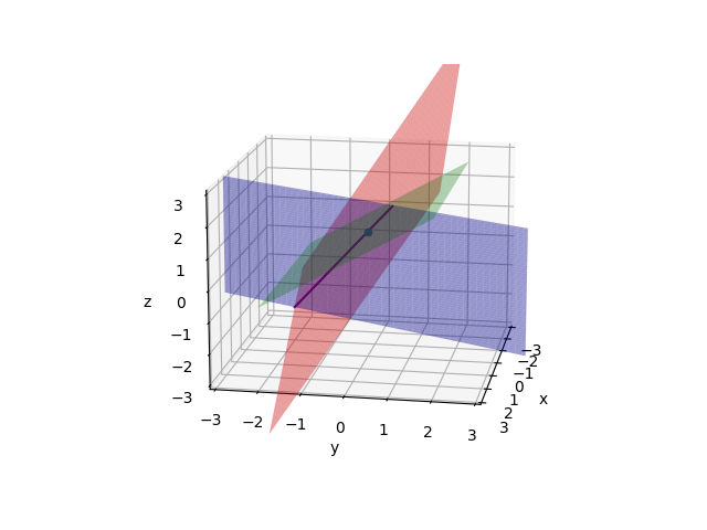
This row picture is complicated. In 4x4 case or higher dimensions, the problem will be more complex, and we have no idea to draw a picture like this.
Then column pictures:
$$
\begin{equation}
x \begin{bmatrix} 2 \\ -1 \\ 0 \end{bmatrix} +
y \begin{bmatrix} -1 \\ 2 \\ -3 \end{bmatrix} +
z \begin{bmatrix} 0 \\ -1 \\ 4 \end{bmatrix} =
\begin{bmatrix} 0 \\ -1 \\ 4 \end{bmatrix}
\end{equation}
$$
Solve this equation, so we can get the linear combination of three vectors. Each vector is a three dimensions one.
Then we can get $x=0, y=0, z=1$.
If we change the $b$. For example $b = x\begin{bmatrix} 1 \\ 1 \\ -3 \end{bmatrix}$. We can also get the linear combination $x=1, y=1, z=0$.
4.3 Can Every Equation Be Solved?
See the last picture. Those three planes are not parallel or special.
Think about this:
Can I solve $A\mathbf{X}=b$ for every $b$?
If we change the x, y and z in this example, we can find that the new vector produced can point at everywhere in this space.
So in linear combination words, the problem is
Do the linear combinations of the columns fill three-dimensional space?
In this example, for the matrix $A$, the answer is yes.
Imagine that if three vectors are in the same plane, and the vector $b$ is out of this plane. Then the combination of three vectors is impossible to produce $b$. In this case, $A$ is called singular matrix. And $A$ would be not invertible.
For non-square matrix like 3x4 matrix, i.e. three equations with four unknowns, it will be introduced later.
4.4 Inverse Matrix
After applying a linear transformation $a$, if we want to undo it, we can look for a matrix $A^{-1}$ to restore the transformation.
For example, $A=\begin{bmatrix} 0 & -1 \\ 1 & 0 \end{bmatrix}$ was a counterclockwise rotation by 90 degrees, then the inverse of A would be a clockwise rotation by 90 degrees: $A^{-1}=\begin{bmatrix} 0 & 1 \\ -1 & 0 \end{bmatrix}$.
Obviously if you multiply a matrix by its inverse, it equals identity matrix. Because after applying the transformation then undo it, the final effect is that nothing happened.
$$
A^{-1}A=AA^{-1}=I
$$
When you have $A^{-1}$, you can multiply it with $A\mathbf{X}=\mathbf{b}$, then it would be:
$$
\begin{align}
A^{-1}A\mathbf{X} &= A^{-1}\mathbf{b} \\
\mathbf{X} &= A^{-1}\mathbf{b}
\end{align}
$$
But when the determinant of the matrix is zero, it squashes space into a smaller dimension. In this case, there is no inverse.
For example, there is a 2x2 matrix squashing space into a line or point. You cannot turn it back into a plane. Because it’s impossible find a linear function to map every vector on the line or point to every vector on the plane.
Properties of Inverse Matrix:
- $(A^{-1})^{-1} = A$
- $(kA)^{-1} = k^{-1}A^{-1} \text{ for any nonzero scalar }k$
- For any invertible nxn matrices A and B, $(AB)^{-1}=B^{-1}A^{-1}$
- $(A^T)^{-1}=(A^{-1})^T$
- $det(A^{-1})=det(A)$
4.5 When does inverse exist
Not all square matrices have inverses. The matrices which have inverses are called invertible or non-singular matrices.
For singular matrices, they have no inverses. And their determinant is 0. And we can find a non-zero vector $x$ with $Ax=0$.
For example, if $A=\begin{bmatrix}1 & 3 \\ 2 & 6\end{bmatrix}$, the columns of A are both on the same line. So every linear combination is on that line and is impossible to get $\begin{bmatrix}1 \\ 0\end{bmatrix}$ or $\begin{bmatrix}0 \\ 1\end{bmatrix}$. That means there is no matrix can be multiplied by $A$ to get $I$.
If $x=\begin{bmatrix}3 \\ -1\end{bmatrix}$, then $Ax=\begin{bmatrix}1 & 3 \\ 2 & 6\end{bmatrix}\begin{bmatrix}3 \\ -1\end{bmatrix}=0$.
Proof: Suppose that we can find a non-zero vector $x$ with $Ax=0$ and A is invertible, then $A^{-1}Ax=Ix=x=0$. So the assumption is false.
4.6 Rank
When the determinant of matrix is zero, for example in 2x2 matrix, it’s possible to find the solution when the solution is on the same line.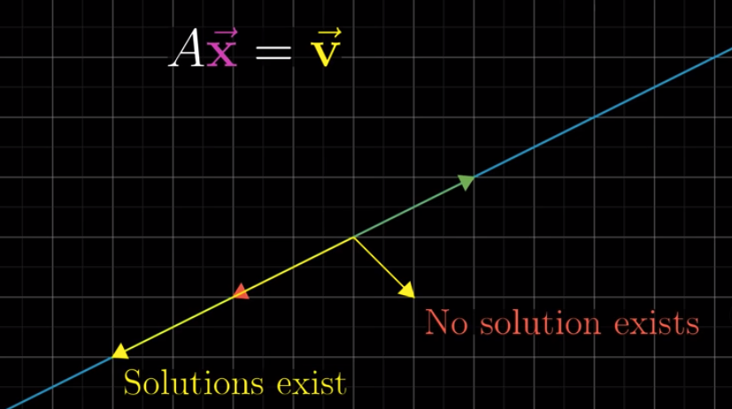
Focus on 3x3 matrix. The transformation may turn the space into a plane, a line, a point, or just stretching or squashing the space.
Rank describes the number of dimensions in all the possible outputs of a linear transformation.
For example, if applying a transformation of 3x3 matrix turns the space into a 2-dimensional plane, the rank of this matrix is 2.
If a 3-D transformation has a non-zero determinant and its output fills all of the 3D space, it has a rank of three. It does not collapse the dimension. In this case, we say the matrix has a full rank.
The set of all possible outputs of $A\vec v$ is called the column space of the matrix $A$.
Notice the zero vector($\begin{bmatrix} 0 \\ 0 \end{bmatrix}$ or $\begin{bmatrix} 0 \\ 0 \\ 0 \end{bmatrix}$…) is always included in the column space, since linear transformation must keep the origin fixed in place.
For a full rank transformation, the only vector that lands at the origin is the zero vector itself.
But for matrices that aren’t full rank, which squashed the space into a smaller dimension, there are a bunch of vectors land on zero. This set of vectors that lands on zero is called the null space or the kernel of the matrix.
In terms of the linear system of equations $A\mathbf{X}=\vec b$, if the vector $\vec b$ happens to be the zero vector, the null space gives you all of the possible solutions to the equation.
5. Elimination with Matrices
5.1 Elimination
Now let’s think about how to solve equations.
For example:
$$
\begin{cases}
x & +2y & +z &= 2 \quad &(1) \\
3x & +8y & +z &= 12 \quad &(2) \\
&\ \ 4y & +z &= 2 \quad &(3)
\end{cases}
$$
And the matrix $A=\begin{bmatrix} 1 & 2 & 1 \\ 3 & 8 & 1 \\ 0 & 4 & 1 \end{bmatrix}$.
If there is an equation, we can accept that if it multiplies a number by or add a number to both sides.
For example:
If $ x + 2 = 3y $, then $ 2 \times (x + 2) = 2 \times 3y $ has the same solution. So does $ 2 \times (x + 2) + z = 2 \times 3y + z $.
So if (1) times a number and then add to (2), it won’t change the solutions of equations. If (1) times $-3$ and then add to (2), we will get $ 2y - 2z = 6$, the $x$ is knocked out. This method is called elimination. It is a common way to solve systems of equations.
If speaking in matrix words, this matrix operation is:
$$
\begin{bmatrix} \boxed{\color{red}{1}} & 2 & 1 \\ 3 & 8 & 1 \\ 0 & 4 & 1 \end{bmatrix}
\xrightarrow{row_2 \ - \ 3row_1}
\begin{bmatrix} \boxed{\color{red}{1}} & 2 & 1 \\ 0 & 2 & -2 \\ 0 & 4 & 1 \end{bmatrix}
$$
The boxed and red number 1 is the key number of this step. We call it pivot.
What about the right-hand vector $b$? Actually Matlab finishes up the left side $A$ and then go back to the right side $b$. So we can do with it later.
In (3), the coefficient of $x$ is already 0. If not, we can eliminate it in the same way.
Next step we can do it again to eliminate the $y$ in (3). In this step the second pivot is 2. Similarly, the thrid pivot is 5
$$
\begin{bmatrix} \boxed{\color{red}{1}} & 2 & 1 \\ 0 & \boxed{\color{green}{2}} & -2 \\ 0 & 4 & 1 \end{bmatrix}
\xrightarrow{row_3 \ - \ 2row_2}
\begin{bmatrix} \boxed{\color{red}{1}} & 2 & 1 \\ 0 & \boxed{\color{green}{2}} & -2 \\ 0 & 0 & \boxed{\color{blue}{5}} \end{bmatrix}
$$
In last step, we get an upper triangular matrix $U=\begin{bmatrix} 1 & 2 & 1 \\ 0 & 2 & -2 \\ 0 & 0 & 5 \end{bmatrix}$
this form is also called echelon form.
So the purpose of elimination is to get from $A$ to $U$.
Note that pivots cannot be 0.
5.2 When does elimination fail?
If the first pivot is 0, does elimination fail? No. In last example, if we exchange the position of (1) and (3), the first pivot will be 0. But the solution of equations won’t be changed. So if the pivots is 0, try exchanging rows.
If $A=\begin{bmatrix} 1 & 2 & 1 \\ 3 & 8 & 1 \\ 0 & 4 & \boxed{-4} \end{bmatrix}$, in last step we will get a matrix $\begin{bmatrix} 1 & 2 & 1 \\ 0 & 2 & -2 \\ 0 & 0 & 0 \end{bmatrix}$. Then the third pivot is 0. It means the equations have no solution. The elimination meets its failure. In this case matrix $A$ would have not been invertible.
5.3 Back substitution
Consider $b$. We can place it to the extra column of $A$ to get an augmented matrix.
$$
[A|b]=
\begin{bmatrix} \begin{array}{ccc | c}
1 & 2 & 1 & 2 \\ 3 & 8 & 1 & 12 \\ 0 & 4 & 1 & 2 \\
\end{array} \end{bmatrix}
$$
Then we do the same operations with this matrix:
$$
\begin{bmatrix} \begin{array}{ccc | c}
1 & 2 & 1 & 2 \\ 3 & 8 & 1 & 12 \\ 0 & 4 & 1 & 2 \\
\end{array} \end{bmatrix}
\xrightarrow{row_2 \ - \ 3row_1}
\begin{bmatrix} \begin{array}{ccc | c}
1 & 2 & 1 & 2 \\ 0 & 2 & -2 & 6 \\ 0 & 4 & 1 & 2 \\
\end{array} \end{bmatrix}
\xrightarrow{row_3 \ - \ 2row_2}
\begin{bmatrix} \begin{array}{ccc | c}
1 & 2 & 1 & 2 \\ 0 & 2 & -2 & 6 \\ 0 & 0 & 5 & -10 \\
\end{array} \end{bmatrix}
$$
$b$ will be a new vector $c=\begin{bmatrix} 2 \\ 6 \\ -10 \end{bmatrix}$
And we can finally get new equations:
$$
\begin{cases}
x & +2y & +z &= 2 \\
&\ \ \ 2y & -2z &= 6 \\
& &\ \ \ 5z &= -10
\end{cases}
$$
Those are the equations $ U \mathbf{X} = c $.
And we can easily figure out that $z=-2, y=1, x=2$.
5.4 Using matrices multiplication to describe the matrices operations
How to use matrix language to describe this operation?
Last lecture we have learnt how to multiply a matrix by a column vector. Here is how to multiply a row vector by a matrix.
$$\begin{equation}
\begin{bmatrix} x & y & z \end{bmatrix}
\begin{bmatrix} a & b & c \\ d & e & f \\ g & h & i \end{bmatrix} =
x \times \begin{bmatrix} a & b & c \end{bmatrix} + y \times \begin{bmatrix} e & f & g \end{bmatrix} + z \times \begin{bmatrix} h & i & j \end{bmatrix}
\end{equation}$$
This is a row operation.
So if the row vector is on the left, the matrix does row operation. If the column vector is on the right, the matrix does column operation.
If a 3x3 matrix is multipied by $I=\begin{bmatrix} 1 & 0 & 0 \\ 0 & 1 & 0 \\ 0 & 0 & 1 \end{bmatrix}$, the matrix would not be changed. $AI = IA = A$. It means this matrix operation do nothing with the matrix $A$. And the matrix $I$ is called identity matrix.
Step 1: Subtract $3 \times row_1$ from $row_2$
$$
\begin{bmatrix} 1 & 0 & 0 \\ -3 & 1 & 0 \\ 0 & 0 & 1 \end{bmatrix}
\begin{bmatrix} 1 & 2 & 1 \\ 3 & 8 & 1 \\ 0 & 4 & 1 \end{bmatrix} =
\begin{bmatrix} 1 & 2 & 1 \\ 0 & 2 & -2 \\ 0 & 4 & 1 \end{bmatrix}
$$
What does this multiplication means? Look at the row 2 of the left matrix. How does it affect the second matrix?
We know $\begin{equation}
\begin{bmatrix} -3 & 1 & 0 \end{bmatrix}
\begin{bmatrix} 1 & 2 & 1 \\ 3 & 8 & 1 \\ 0 & 4 & 1 \end{bmatrix} =
-3 \times \begin{bmatrix} 1 & 2 & 1 \end{bmatrix} + 1 \times \begin{bmatrix} 3 & 8 & 1 \end{bmatrix} + 0 \times \begin{bmatrix} 0 & 4 & 1 \end{bmatrix} =
\begin{bmatrix} 0 & 2 & -2 \end{bmatrix}
\end{equation}$
So $\begin{bmatrix}-3 & 1 & 0\end{bmatrix}$ means $-3 \times row_1 + 1 \times row_2 + 0 \times row_3$ produces the second row $\begin{bmatrix}0 & 2 & -2\end{bmatrix}$ of new matrix.
And the simple matrix $E_{21}=\begin{bmatrix} 1 & 0 & 0 \\ -3 & 1 & 0 \\ 0 & 0 & 1 \end{bmatrix} $ which is used to operate the matrix $A$ is called Elementary Matrix.
$E_{21}$ means it will change the number to 0 on the position of row 2 and column 1.
Step 2: Subtract $2 \times row_2$ from $row_3$.
$$
\begin{bmatrix} 1 & 0 & 0 \\ 0 & 1 & 0 \\ 0 & -2 & 1 \end{bmatrix}
\begin{bmatrix} 1 & 2 & 1 \\ 0 & 2 & -2 \\ 0 & 4 & 1 \end{bmatrix} =
\begin{bmatrix} 1 & 2 & 1 \\ 0 & 2 & -2 \\ 0 & 0 & 5 \end{bmatrix}
$$
We use $E_{32}$ to represent the left matrix.
These two operations can be written as $E_{32}(E_{21}A)=U$
We use two elementary matrices to produce the matrix $U$. Can we use only one matrix to do that? The answer is yes.
$$E_{32}(E_{21}A)==(E_{32}E_{21})A=EA=U,\\
\mathrm{composition\ matrix}\ E=E_{32}E_{21}$$
This method to change the parentheses is called associative law.
The composition matrix is the multiplication of two matrices. It mixes two transformations into one. And this is the meaning of matrices multiplication.
The elementary matrix to add row(j) multiplied by a number(k) to another row(i) can be written as
$$
\begin{bmatrix}
1 & & & & & & \\
& \ddots & & & & & \\
& & 1 & \cdots & k & & \\
& & & \ddots & \vdots & & \\
& & & & 1 & & \\
& & & & & \ddots & \\
& & & & & & 1
\end{bmatrix}
$$
k is on the (i, j)
The elementary matrix to scale row(i) by k:
$$
\begin{bmatrix}
1 & & & & & & \\
& \ddots & & & & & \\
& & 1 & & & & \\
& & & k & & & \\
& & & & 1 & & \\
& & & & & \ddots & \\
& & & & & & 1
\end{bmatrix}
$$
k is on the row(i)
5.5 Permutation Matrix
Another elementary matrix that exchanges two rows is called Permutation Matrix.
For example, if we want to exchange two rows of $\begin{bmatrix} a & b \\ c & d \end{bmatrix}$, what matrix can we use?
$$
\begin{bmatrix} 0 & 1 \\ 1 & 0 \end{bmatrix}
\begin{bmatrix} a & b \\ c & d \end{bmatrix} =
\begin{bmatrix} c & d \\ a & b \end{bmatrix}
$$
How if we want to exchange two columns of matrix? Put the permutation matrix on the right.
$$
\begin{bmatrix} a & b \\ c & d \end{bmatrix}
\begin{bmatrix} 0 & 1 \\ 1 & 0 \end{bmatrix} =
\begin{bmatrix} b & a \\ d & c \end{bmatrix}
$$
According to this two examples, we know that $AB$ is not the same as $BA$. So the order of the matrix multiplication is important.
To change the row on i and j, just change the these two rows of the identity matrix. Then the modified identity matrix is the elementary matrix we need.
$$
\begin{bmatrix}
1 & & & & & & & & & & \\
& \ddots & & & & & & & & & \\
& & 1 & & & & & & & & \\
& & & 0 & & & & 1 & & & \\
& & & & 1 & & & & & & \\
& & & & & \ddots & & & & & \\
& & & & & & 1 & & & & \\
& & & 1 & & & & 0 & & & \\
& & & & & & & & 1 & & \\
& & & & & & & & & \ddots & \\
& & & & & & & & & & 1
\end{bmatrix}
$$
5.6 How to get from U back to A
See the matrix $\begin{bmatrix} 1 & 0 & 0 \\ -3 & 1 & 0 \\ 0 & 0 & 1 \end{bmatrix}$. It subtract $3 \times row_1$ from $row_2$. How to undo this operation?
We know $IA=A$. So if we can find out a matrix $E^{-1}$ so that $E^{-1}E=I$, then $E^{-1}EA=IA=A$.
The matrix $E^{-1}$ is called $E$ inverse.
$$
\begin{bmatrix} 1 & 0 & 0 \\ 3 & 1 & 0 \\ 0 & 0 & 1 \end{bmatrix}
\begin{bmatrix} 1 & 0 & 0 \\ -3 & 1 & 0 \\ 0 & 0 & 1 \end{bmatrix}=
\begin{bmatrix} 1 & 0 & 0 \\ 0 & 1 & 0 \\ 0 & 0 & 1 \end{bmatrix}
$$
5.7 Using Elimination to get $A^{-1}$
$A=\begin{bmatrix}1 & 3 \\ 2 & 7\end{bmatrix}$ for example, suppose $A^{-1}=\begin{bmatrix}a & b \\ c & d\end{bmatrix}$, then $\begin{bmatrix}1 & 3 \\ 2 & 7\end{bmatrix}\begin{bmatrix}a & c \\ b & d\end{bmatrix}=\begin{bmatrix}1 & 0 \\ 0 & 1\end{bmatrix}$. We can get a system of equations:$
\begin{cases}
\begin{bmatrix}1 & 3 \\ 2 & 7\end{bmatrix}\begin{bmatrix}a \\ b\end{bmatrix}=\begin{bmatrix}1 \\ 0\end{bmatrix} \\
\begin{bmatrix}1 & 3 \\ 2 & 7\end{bmatrix}\begin{bmatrix}c \\ d\end{bmatrix}=\begin{bmatrix}0 \\ 1\end{bmatrix}
\end{cases}$
Gauss-Jordam(Solve 2 equations at once):
Stick the I to the right of A, making it an augmented matrix:$
[\color{red}A\color{black}|\color{blue}I\color{black}]=
\begin{bmatrix}\begin{array}{cc | cc}
1 & 3 & 1 & 0 \\
2 & 7 & 0 & 1
\end{array}\end{bmatrix}$.
Then transform it into $[I|E]$ by elimination.
$$
\begin{bmatrix}\begin{array}{cc | cc}
1 & 3 & 1 & 0 \\
2 & 7 & 0 & 1
\end{array}\end{bmatrix}
\xrightarrow[E_{21}]{row_2 \ - \ 2row_1}
\begin{bmatrix}\begin{array}{cc | cc}
1 & 3 & 1 & 0 \\
0 & 1 & -2 & 1
\end{array}\end{bmatrix}
\xrightarrow[E_{12}]{row_1 \ - \ 3row_2}
\begin{bmatrix}\begin{array}{cc | cc}
1 & 0 & 7 & -3 \\
0 & 1 & -2 & 1
\end{array}\end{bmatrix}
$$
See the left side. The matrix operation $E=E_{21}E_{12}$ makes $\color{red} A$ become $I$. So $E\color{red}A\color{black}=I$. And the right side $\color{blue}I$ becomes $E$ because $E\color{blue}I\color{black}=E$. Then $E=A^{-1}$.
6. Nonsquare Matrices, Dot Products, Cross Products and Solving System of Linear Equations
6.1 Non-square Matrices
Think about matrices that are not square. What’s the meaning of them? How to use them?
For example, there is a 3x2 metrix $\begin{bmatrix} 3 & 1 \\ 4 & 1 \\ 5 & 2 \end{bmatrix}$
$$
\begin{equation}
\begin{bmatrix} 3 & 1 \\ 4 & 1 \\ 5 & 2 \end{bmatrix}
\begin{bmatrix} 2 \\ 3 \end{bmatrix}
=
\begin{bmatrix} 9 \\ 11 \\ 6 \end{bmatrix}
\end{equation}
$$
If we multiply it by a 2-dimensional vector, it produces a 3-dimensional vector. The matrix tells where $\hat i$ lands and where $\hat j$ lands.
$$
\begin{align}
\color{green} \text{where } &\color{green}\hat{i} \text{ lands} \\
&\color{black}\begin{bmatrix}
\color{green} 3 & \color{red} 1 \\
\color{green} 4 & \color{red} 1 \\
\color{green} 5 & \color{red} 2
\end{bmatrix} \\
&\color{red}\text{where } \color{red}\hat{j} \text{ lands}
\end{align}
$$
Likewise, if there is a 2x3 matrix with two rows and three columns, the three columns indicate that it starts with a space with three basis vectors, and the two rows indicate that the landing spot for each of those basis vectors is described with only two coordinates, so they must be landing in two dimensions.
$$
\begin{equation}
\begin{bmatrix} 3 & 1 & 4 \\ 1 & 5 & 2 \end{bmatrix}
\begin{bmatrix} 3 \\ 1 \\ 2 \end{bmatrix}
=
\begin{bmatrix} 18 \\ 12 \end{bmatrix}
\end{equation}
$$
So it turns a 3-D vector into a 2-D vector.
6.2 Dot Products
6.2.1 Geometrical Intuition of Dot Product
If there is a 2x1 transformation matrix, it turns 2-D vector2 into one dimension. One-dimensional space is just the number line, so the matrix turns vectors into numbers.
Dot product of two vectors $\vec v$, $\vec u$ is described as the multiplication between the length of $\vec u$ and the length of the vector $\vec w$. $\vec w$ is the vector $\vec u$ projecting onto $\vec v$.
If the projection of $\vec u$ is pointing in the opposite direction from $\vec v$, the dot product will be negative.
When two vectors are perpendicular, meaning the projection of one onto the other is the zero vector, their dot product is 0.
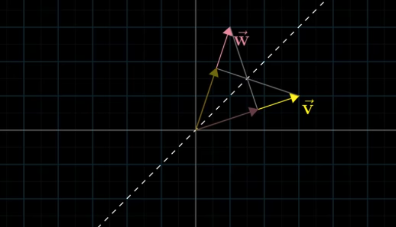
Obviously the order of $\vec u$ and $\vec v$ doesn’t affect the result: $\vec u \cdot \vec v = \vec v \cdot \vec u$
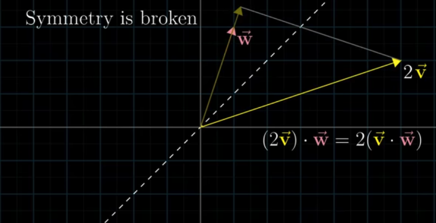
Geometrically, it can be described as symmetric, i.e. (length of projection $\vec u$)(length of $\vec v$)=(length of $\vec u$)(length of projection $\vec v$).
If there are two vectors which have the same length, they are obviously symmetric. And it’s a certainty that $\vec u \cdot \vec v = \vec v \cdot \vec u$ for symmetry.
If they are asymmetric, for example, scaling $\vec v$ by 2, the projection of $w$ won’t be changed. So the result is twice the dot product of $\vec u$ and $\vec v$.
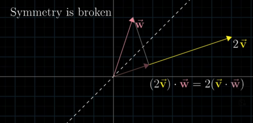
Thinking about $\vec v$ getting projected onto $\vec w$. In this case, the length of projection gets scaled by 2. The overall effect is still to just double the dot product.
6.2.2 Numerical Computation and its Geometrical Meaning
Numerically compute:
$$
\vec u \cdot \vec v = \sum_{i=1}^n \vec u_i \vec v_i
$$
What’s the connection between this numerical process and geometrical conception?
If there is a 1x2 matrix that transforms the vector into a number:
$$
\begin{equation}
\begin{bmatrix} 1 & -2 \end{bmatrix}
\begin{bmatrix} 4 \\ 3 \end{bmatrix}
=
4 \cdot 1 + 3 \cdot (-2)
=
-2
\end{equation}
$$
This numerical operation of multiplying a 1x2 matrix by a vector feels like taking the dot product of two vectors.
The matrix tells where $\hat i$ and $\hat j$ lands onto the number line, and the vector describes the coefficient of $\hat i$ and $\hat j$. And the final 1-dimensional vector on the number line, which is a number, is the result of dot product.
6.3 Cross Products
The cross product of two vector $\vec v$ and $\vec w$ in 3-D space is defined as
$$
\begin{equation}
\begin{bmatrix} v_1 \\ v_2 \\ v_3 \end{bmatrix}
\times
\begin{bmatrix} w_1 \\ w_2 \\ w_3 \end{bmatrix}
=
\begin{bmatrix}
v_2 \cdot w_3 - w_2 \cdot v_3 \\
v_3 \cdot w_1 - w_3 \cdot v_1 \\
v_1 \cdot w_2 - w_1 \cdot v_2
\end{bmatrix}
\end{equation}
$$
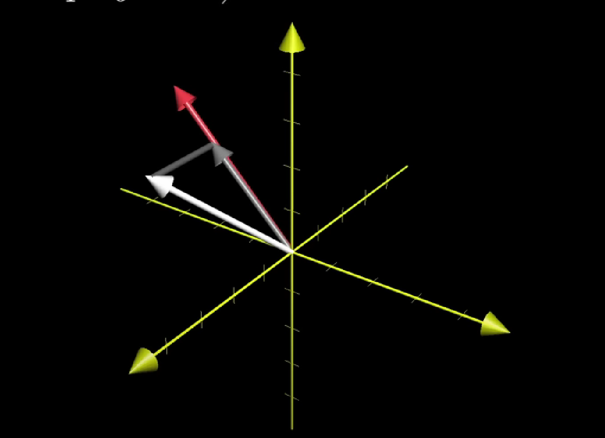
The outcome vector is perpendicular to the parallelogram spanned up by $\vec v$ and $\vec w$, and the direction follows the right-hand rule.
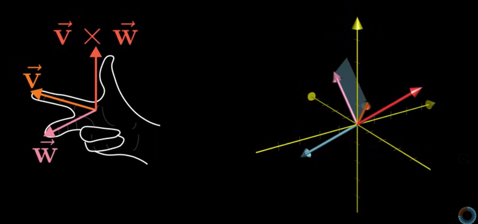
The length of the outcome vector is the area of the parallelogram spanned up by $\vec v$ and $\vec w$.
- $\vec v \cdot (\vec \times \vec w) = 0$
- $\vec w \cdot (\vec \times \vec w) = 0$
- $||(\vec v \times \vec w) = ||\vec v|| \times ||\vec w|| \times \sin (\theta)$
There is a notation trick:
$$
\begin{equation}
\color{red} \begin{bmatrix} v_1 \\ v_2 \\ v_3 \end{bmatrix}
\color{black} \times
\color{blue} \begin{bmatrix} w_1 \\ w_2 \\ w_3 \end{bmatrix}
\color{black}
=
\begin{vmatrix}
\hat i & \color{red} v_1 & \color{blue} w_1 \\
\hat j & \color{red} v_2 & \color{blue} w_2 \\
\hat k & \color{red} v_3 & \color{blue} w_3
\end{vmatrix}
=
\hat{i}(\color{red}v_2 \color{black}\cdot \color{blue}w_3 \color{black}- \color{blue}v_3 \color{black}\cdot \color{red}w_2) \color{black} +
\hat{j}(\color{red}v_3 \color{black}\cdot \color{blue}w_1 \color{black}- \color{blue}v_1 \color{black}\cdot \color{red}w_3) \color{black} +
\hat{k}(\color{red}v_1 \color{black}\cdot \color{blue}w_2 \color{black}- \color{blue}v_2 \color{black}\cdot \color{red}w_1)
\end{equation}
$$
6.4 Deep Dive into Cross Products
So what’s the meaning of the cross product? Why defining a vector that’s perpendicular to the plane spanned up by two vectors?
If the third vector $\vec u = \begin{bmatrix} x \\ y \\ z \end{bmatrix}$ is variable, the volume of the parallelepiped will be variable.
$$
\begin{align}
the\ volume\ of\ the\ parallelepipied &=
\begin{vmatrix}
x & \color{red}v_1 & \color{blue}w_1 \\
y & \color{red}v_2 & \color{blue}w_2 \\
z & \color{red}v_3 & \color{blue}w_3
\end{vmatrix} \\
&=
x(\color{red}v_2 \color{black}\cdot \color{blue}w_3 \color{black}- \color{blue}v_3 \color{black}\cdot \color{red}w_2) \color{black} +
y(\color{red}v_3 \color{black}\cdot \color{blue}w_1 \color{black}- \color{blue}v_1 \color{black}\cdot \color{red}w_3) \color{black} +
z(\color{red}v_1 \color{black}\cdot \color{blue}w_2 \color{black}- \color{blue}v_2 \color{black}\cdot \color{red}w_1)
\end{align}
$$
We can see the result is similar to the cross product of $\vec v$ and $\vec w$. The $x$, $y$ and $z$ are unknowns. We can pack the coefficient of each unknown into $\vec p$.
$$
\begin{align}
p_1 &= \color{red}v_2 \color{black}\cdot \color{blue}w_3 \color{black}- \color{blue}v_3 \color{black}\cdot \color{red}w_2 \\
p_2 &= \color{red}v_3 \color{black}\cdot \color{blue}w_1 \color{black}- \color{blue}v_1 \color{black}\cdot \color{red}w_3 \\
p_3 &= \color{red}v_1 \color{black}\cdot \color{blue}w_2 \color{black}- \color{blue}v_2 \color{black}\cdot \color{red}w_1 \\
\end{align}
$$
Then
$$
\begin{vmatrix}
x & \color{red}v_1 & \color{blue}w_1 \\
y & \color{red}v_2 & \color{blue}w_2 \\
z & \color{red}v_3 & \color{blue}w_3
\end{vmatrix}
=
p_1 x + p_2 y + p_3 z
$$
The result looks like dot product, so we can pack $p_1$, $p_2$ and $p_3$ into a vector:
$$
\begin{bmatrix}
p_1 \\
p_2 \\
p_3
\end{bmatrix}
\cdot
\begin{bmatrix}
x \\
y \\
z
\end{bmatrix}
=
\begin{vmatrix}
x & \color{red}v_1 & \color{blue}w_1 \\
y & \color{red}v_2 & \color{blue}w_2 \\
z & \color{red}v_3 & \color{blue}w_3
\end{vmatrix}
$$
Then the question becomes, what 3-D vector $\vec p$ has the special property, that when you take a dot product between $\vec p$ and some vector $\begin{bmatrix} x \\ y \\ z \end{bmatrix}$, it gives the same result as plugging in the vector $\begin{bmatrix} x \\ y \\ z \end{bmatrix}$ to the first column of a matrix whose other two columns have the coordinates of $\vec v$ and $\vec w$, then computing the determinant.
Geometrically, the question is, what 3-D vector $\vec p$ has the special property, that when you take a dot product between $\vec p$ and some vector $\begin{bmatrix} x \\ y \\ z \end{bmatrix}$, it gives the same result as if you took the signed volume of a parallelepiped defined by this vector $\begin{bmatrix} x \\ y \\ z \end{bmatrix}$ along with $\vec v$ and $\vec w$.
We know determinant of a 3x3 matrix, i.e. the pack of three vectors, is the volume of parallelepiped. And a dot product of two 3-D vectors is related to the projection of one vector.
The volume of a parallelepiped, is the area of the parallelogram times the height of the parallelepiped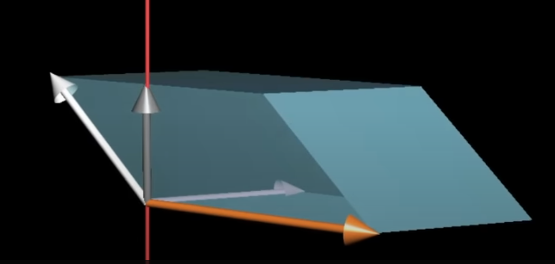
In other words, the way our linear function works on a given vector is to project that vector onto a line that’s perpendicular to both $\vec v$ and $\vec w$, then to multiply the length of that projection by the area of the parallelogram spanned by $\vec v$ and $\vec w$.
But it’s the same thing as taking a dot product between $\begin{bmatrix} x \\ y \\ z \end{bmatrix}$ and a vector that’s perpendicular to $\vec v$ and $\vec w$ with a length equal to the area of parallelogram.
$$
\begin{align}
& (\text{area of parallelogram})\times(\text{the height})=(\begin{bmatrix} x \\ y \\ z \end{bmatrix} \cdot \vec p) \\
& \vec p \text{ is perpendicular to } \vec v \text{ and } \vec w \text{, with a length equals to that parallelogram}
\end{align}
$$
This is the fundamental reason why the computation and the geometric interpretation of the cross product are related.
6.5 Mixed Products
Mixed product of three vectors
$$
(\vec a, \vec b, \vec c) = (\vec a \times \vec b) \cdot \vec c =
\begin{vmatrix}
a_1 & b_1 & c_1 \\
a_2 & b_2 & c_2 \\
a_3 & b_3 & c_3
\end{vmatrix}
$$
The number of mixed product represents the signed volume of the parallelepiped spanned by three vectors $\vec a$, $\vec b$ and $\vec c$.
If the mixed product is zero, meaning the volume of that parallelepiped is zero, three vectors $\vec a$, $\vec b$ and $\vec c$ lie on the same plane.
6.6 Solving System of Linear Equations
6.6.1 Solving $Ax=0$
The systems of equations like $Ax=0$ are called homogeneous system of linear equations.
For example,
$$
\begin{cases}
x_1 &+ 2x_2 &+ 3x_3 &= 0 \\
2x_1 &+ 4x_2 &+ 6x_3 &= 0 \\
2x_1 &+ 6x_2 &+ 8x_3 &= 0 \\
2x_1 &+ 8x_2 &+ 10x_3 &= 0
\end{cases}
$$
For these equations, obviously there is a special solution $\begin{bmatrix} 0 \\ 0 \\ 0 \\ 0 \end{bmatrix}$ because all the right-hand constants b are 0. This special solution is call trivial solution.
The matrix and the eliminated version of that matrix:
$$
\begin{equation}
A=
\begin{bmatrix}
1 & 2 & 2 \\
2 & 4 & 6 \\
2 & 6 & 8 \\
2 & 8 & 10
\end{bmatrix}
\xrightarrow{eliminate}
\begin{bmatrix}
\boxed{1} & 2 & 3 \\
0 & \boxed{2} & 2 \\
0 & 0 & 0 \\
0 & 0 & 0
\end{bmatrix}
\end{equation}
$$
There is 2 pivot variables(boxed number $\boxed{1}$ and $\boxed{2}$). The rank of the matrix A is 2.
The columns in which pivot variables locate are called pivot columns, and other columns are called free columns. The variables in free columns are called free variables. The amount of free variables is $n-r=3-2=1$.
The equations become
$$
\begin{cases}
x_1 &+ 2x_2 &+ 3x_3 &= 0 \\
&\quad 2x_2 &+ 2x_3 &= 0 \\
\end{cases}
$$
We can let the free variable $x_3=1$, then solve the equations and get $x=\begin{bmatrix} -1 \\ -1 \\ 1 \end{bmatrix}$
If we scale the solution $x$ by a constant $c$, then $cx$ is also the solution of the equation.
So the nontrivial solution is $x=c\begin{bmatrix} -1 \\ -1 \\ 1 \end{bmatrix}$
Take another example,
$$
\begin{cases}
x_1 &+ 2x_2 &+ 2x_3 &+ 2x_4 &= 0 \\
2x_1 &+ 4x_2 &+ 6x_3 &+ 8x_4 &= 0 \\
3x_1 &+ 6x_2 &+ 8x_3 &+ 10x_4 &= 0
\end{cases}
$$
The matrix and the eliminated version of that matrix:
$$
\begin{equation}
A=
\begin{bmatrix}
1 & 2 & 2 & 2 \\
2 & 4 & 6 & 8 \\
3 & 6 & 8 & 10
\end{bmatrix}
\xrightarrow{eliminate}
\begin{bmatrix}
\boxed{1} & 2 & 2 & 2 \\
0 & 0 & \boxed{2} & 4 \\
0 & 0 & 0 & 0
\end{bmatrix}
\end{equation}
$$
There is 2 pivot variables(boxed number $\boxed{1}$ and $\boxed{2}$). The rank of the matrix A is 2.
In this example, the pivot columns are column 1 and 3, and the free columns are column 2 and 4.
Let one of the free variable be 1 and others be 0.
When $x_2=1$ and $x_4=0$, solve the equations, and then we can get $x=\begin{bmatrix} -2 \\ 1 \\ 0 \\ 0 \end{bmatrix}$.
When $x_2=0$ and $x_4=1$, solve the equations, and then we can get $x=\begin{bmatrix} 2 \\ 0 \\ -2 \\ 1 \end{bmatrix}$.
In each case, each $x$ times a constant $c$ is still the solution of equations.
So the solution set of the equations is the set of $x=c_1\begin{bmatrix} -2 \\ 1 \\ 0 \\ 0 \end{bmatrix}$ and $x=c_2\begin{bmatrix} 2 \\ 0 \\ -2 \\ 1 \end{bmatrix}$.
What’s more, the linear combination of the solution set is also the solution of the equations.
You may confuse that the special solution $x=c_2\begin{bmatrix} 0 \\ 1 \\ -2 \\ 1 \end{bmatrix}$ is also the solution of equations, but each solution in solution set cannot be scaled to produce it. Actually, it’s the linear combination when $c_1=1$ and $c_2=1$.
The linear combination of the two solution contains all the special solutions, including nontrivial solutions and trivial solutions(when $c_1=c_2=0$).
So the solution of the equations is $x=c_1\begin{bmatrix} -2 \\ 1 \\ 0 \\ 0 \end{bmatrix}+c_2\begin{bmatrix} 2 \\ 0 \\ -2 \\ 1 \end{bmatrix}$.
Generally, for system of equations with n unknowns(or mxn matrix), let $rank(A)=r$. Certainly $r \leqslant n$.
If $r=n$, then there is no free variable in equations. So in this case there is only a trivial solution $x=\begin{bmatrix} 0 \\ 0 \\ \vdots \\ 0 \end{bmatrix}$.
If $r<n$, then there are $(n-r)$ nontrivial equation(s)
$$
\begin{cases}
\quad\eta_1 &= c_1\begin{bmatrix} a_{11} & a_{12} & \cdots & a_{1r} & 1 & 0 & 0 & \cdots & 0 \end{bmatrix}^T \\
\quad\eta_2 &= c_2\begin{bmatrix} a_{21} & a_{22} & \cdots & a_{2r} & 0 & 1 & 0 & \cdots & 0 \end{bmatrix}^T \\
\quad\eta_3 &= c_3\begin{bmatrix} a_{31} & a_{32} & \cdots & a_{3r} & 0 & 0 & 1 & \cdots & 0 \end{bmatrix}^T \\
\quad\vdots \\
\eta_{n-r} &= c_{n-r,1}\begin{bmatrix} a_{n-r,1} & a_{n-r,2} & \cdots & a_{n-r,r} & 0 & 0 & 0 & \cdots & 1 \end{bmatrix}^T
\end{cases}
$$
Solutions $\eta_1,\ \eta_2,\ \cdots,\ \eta_n$ are linear independent. And every special solution of the equations can be described as the linear combination of them.
The solution of $Ax=0$ is also called the solution in the nullspace.
6.6.2 Non-homogeneous System of Linear Equations
For example,
$$
\begin{cases}
x_1 &+ 2x_2 &+ 2x_3 &+ 2x_4 &= b_1 \\
2x_1 &+ 4x_2 &+ 6x_3 &+ 8x_4 &= b_2 \\
3x_1 &+ 6x_2 &+ 8x_3 &+ 10x_4 &= b_3
\end{cases}
$$
The augmented matrix and elimination:
$$
\begin{equation}
\begin{bmatrix}
\begin{array}{cccc:c}
1 & 2 & 2 & 2 & b_1 \\
2 & 4 & 6 & 8 & b_2 \\
3 & 6 & 8 & 10 & b_3
\end{array}
\end{bmatrix}
\xrightarrow{eliminate}
\begin{bmatrix}
\begin{array}{cccc:c}
1 & 2 & 2 & 2 & b_1 \\
0 & 0 & 2 & 4 & b_2 - 2b_1 \\
0 & 0 & 0 & 0 & b_3 - b_2 - b_1
\end{array}
\end{bmatrix}
\end{equation}
$$
Obviously $Ax=b$ is solvable when $b_3-b_2-b_1=0$.
Generally, $Ax=b$ is solvable when b is in $C(A)$.
In other words, if a combination of the rows of A gives zero rows, then the same combination of entries of b must give 0.
In order to get the complete solution of the equations, we can get the particular solution $Ax_p=b$ and the special solution in the nullspace $Ax_n=0$, then add them together: $A(x_p+x_n)=b$.
Because $Ax_n=0$ and $Ax_p=b$, we can get $A(x_p+x_n)=Ax_p + Ax_n = b + 0 = b$.
Step 1, to get the special solution $x_n$, we let all free variables be zero, then solve the equations.
In the example above, the free variables are $x_2$ and $x_4$, we let $x_2 = x_4 = 0$. Solve the equations, we can get $x_p=\begin{bmatrix} -2 \\ 0 \\ \cfrac{3}{2} \\ 0 \end{bmatrix}$.
Step 2, get the solution in the nullspace.
Let $x_2=1$ and $x_4=0$, then solve $Ax=0$, we get $x=\begin{bmatrix} -2 \\ 1 \\ 0 \\ 0 \end{bmatrix}$.
Let $x_2=0$ and $x_4=1$, then solve $Ax=0$, we get $x=\begin{bmatrix} 2 \\ 0 \\ -2 \\ 1 \end{bmatrix}$.
Step 3, add the particular solution and special solutions together.
$$
x =
\begin{bmatrix} -2 \\ 0 \\ \cfrac{3}{2} \\ 0 \end{bmatrix} +
c_1\begin{bmatrix} -2 \\ 1 \\ 0 \\ 0 \end{bmatrix} +
c_2\begin{bmatrix} 2 \\ 0 \\ -2 \\ 1 \end{bmatrix}
$$
Since in the nullspace, no matter how the linear combination is, $Ax$ always be zero. And we get all solutions in nullspace, meaning we can reach every solution by $x_p+x_n$, so this solution of equations is the complete solution.
Generally, for system of equations with n unknowns(or mxn matrix), let $rank(A)=r$. Certainly $r \leqslant n$.
If $r=n$, then there is no free variable in equations, meaning the nullspace is only the zero vector. So there is only one special solution or no solution.
If $r<n$, we just let every free variables equal zero to get one of the particular solution. Then get the solution in nullspace, add them together to get the complete solution.
6.6.3 Solvability of $Ax=b$
If $A$ is a mxn matrix, the rank of $A$ is $r$, then we call $A$ has a full row rank if $r=m$.
When $A$ has a full row rank, $Ax=b$ is solvable for any $b$. Because when $n>m$, there are $(n-r)$ free variable(s). When $n=m$, the matrix has a full rank, so it’s solvable.
7. Cramer’s Rule
As a method to solve the linear systems of equations, Cramer’s rule is not the best way(Gaussian elimination for example will be faster). But the relationship between computation and geometry in Cramer’s rule is also worth thinking about.
Computation:
To solve the system of equations:
$$
\begin{cases}
a_{11} x + a_{12} y + a_{13} z = \color{blue}b_1 \\
a_{21} x + a_{22} y + a_{23} z = \color{blue}b_2 \\
a_{31} x + a_{32} y + a_{33} z = \color{blue}b_3
\end{cases}
$$
Matrix form:
$$
\begin{bmatrix}
a_{11} & a_{12} & a_{13} \\
a_{21} & a_{22} & a_{23} \\
a_{31} & a_{32} & a_{33}
\end{bmatrix}
\begin{bmatrix} x \\ y \\ z \end{bmatrix}
=
\begin{bmatrix} \color{blue}b_1 \\ \color{blue}b_2 \\ \color{blue}b_3 \end{bmatrix}
$$
For the matrix whose determinant is not zero:
$$
\begin{equation}
x = \cfrac{
\begin{vmatrix}
\color{blue}b_{1} & a_{12} & a_{13} \\
\color{blue}b_{2} & a_{22} & a_{23} \\
\color{blue}b_{3} & a_{32} & a_{33}
\end{vmatrix}
}{
\begin{vmatrix}
a_{11} & a_{12} & a_{13} \\
a_{21} & a_{22} & a_{23} \\
a_{31} & a_{32} & a_{33}
\end{vmatrix}
},
y = \cfrac{
\begin{vmatrix}
a_{11} & \color{blue}b_{1} & a_{13} \\
a_{21} & \color{blue}b_{2} & a_{23} \\
a_{31} & \color{blue}b_{3} & a_{33}
\end{vmatrix}
}{
\begin{vmatrix}
a_{11} & a_{12} & a_{13} \\
a_{21} & a_{22} & a_{23} \\
a_{31} & a_{32} & a_{33}
\end{vmatrix}
},
z = \cfrac{
\begin{vmatrix}
a_{11} & a_{12} & \color{blue}b_{1} \\
a_{21} & a_{22} & \color{blue}b_{2} \\
a_{31} & a_{32} & \color{blue}b_{3}
\end{vmatrix}
}{
\begin{vmatrix}
a_{11} & a_{12} & a_{13} \\
a_{21} & a_{22} & a_{23} \\
a_{31} & a_{32} & a_{33}
\end{vmatrix}
}
\end{equation}
$$
It also works for systems of larger number of unknowns and the same number of equations. But a smaller example is nicer for the sake of simplicity.
$$
\begin{bmatrix}
\color{green} 3 & \color{red}2 \\
\color{green}-1 & \color{red}2
\end{bmatrix}
\begin{bmatrix}
x \\
y
\end{bmatrix}
=
\begin{bmatrix}
\color{blue}-4 \\
\color{blue}-2
\end{bmatrix}
$$
The question is, which the input vector $\begin{bmatrix} x \\ y \end{bmatrix}$ is going to land on the output $\begin{bmatrix} \color{blue}-4 \\ \color{blue}-2 \end{bmatrix}$ after transformation.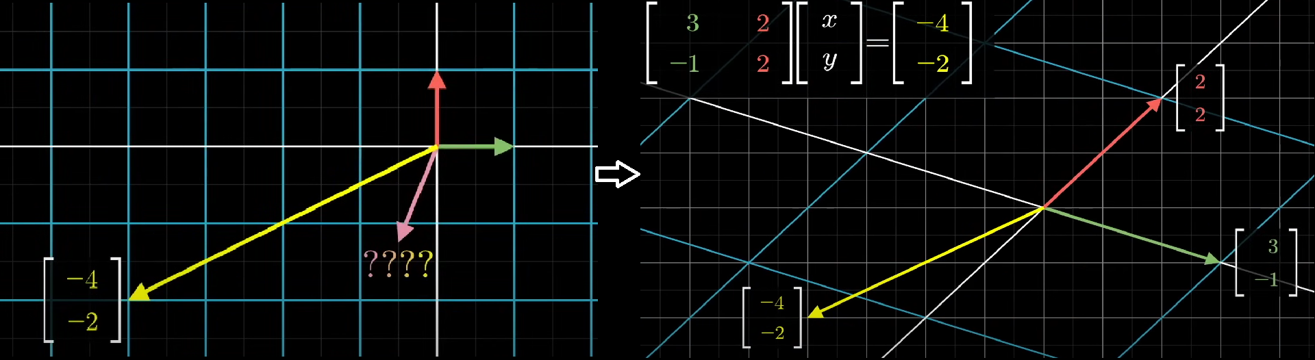
One way to think about is to find a linear combination.
$$
x \begin{bmatrix} \color{green} 3 \\ \color{green}-1 \end{bmatrix} +
y \begin{bmatrix} \color{red} 2 \\ \color{red}2 \end{bmatrix} =
\begin{bmatrix} \color{blue} -4 \\ \color{blue}-2 \end{bmatrix}
$$
But it’s not easy to calculate when the number of unknowns and equations goes high.
See another idea. Take the parallelogram defined by the first basis vector $\hat i$ and the unknown input vector $\begin{bmatrix} x \\ y \end{bmatrix}$. The are of the parallelogram is the base 1 times the height perpendicular to that base, which is the y-coordinate. So the area of the parallelogram is y. Notice that the area is signed. When y is negative, then the area will be negative as well.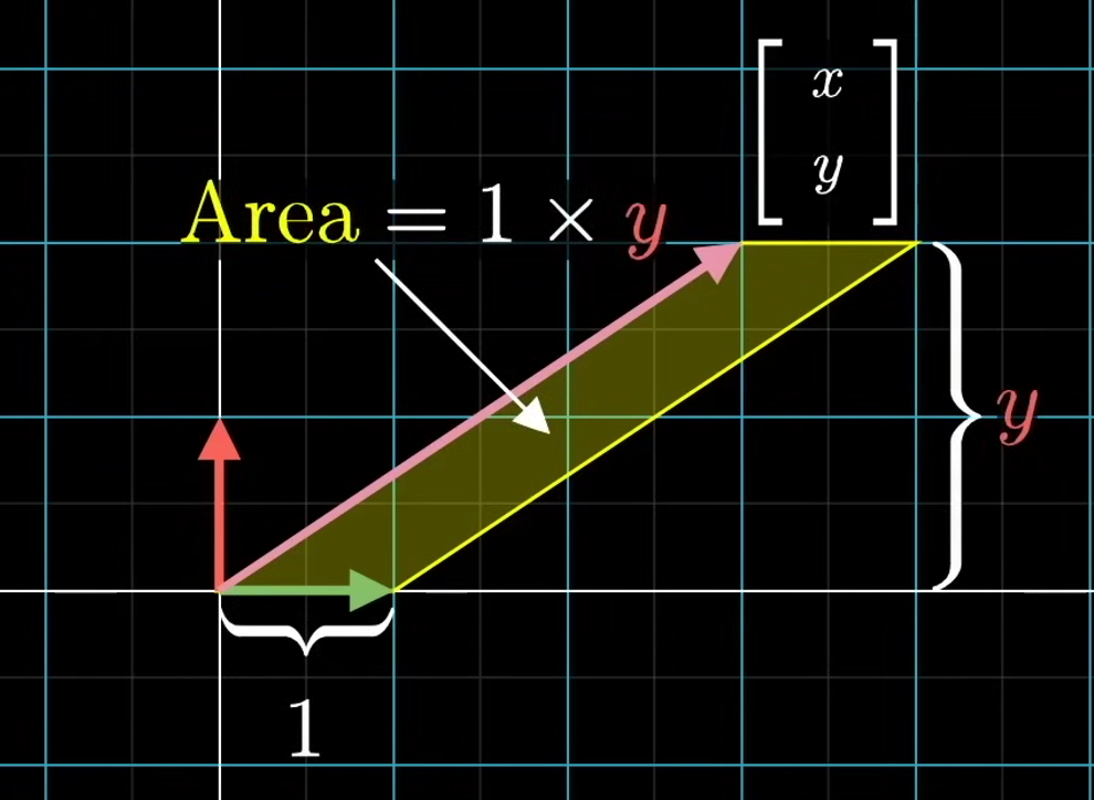
And symmetrically, if you look at the parallelogram spanned up by the unknown vector and $\hat j$, the area will be x.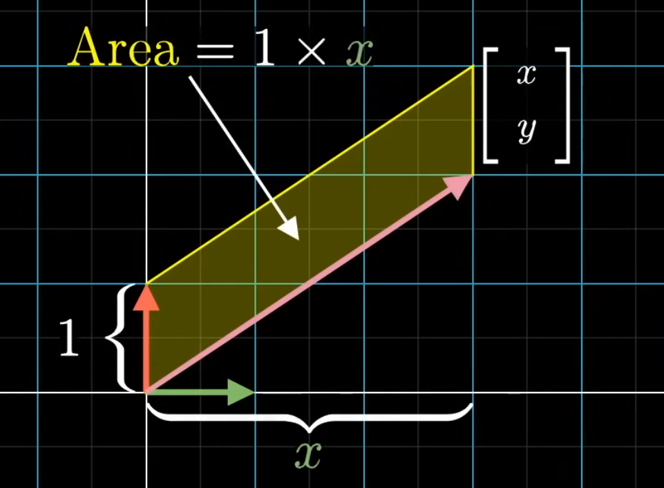
Then the question is:
$$
\begin{bmatrix} \color{green}1 & \color{red}0 \\ \color{green}0 & \color{red}1 \end{bmatrix}
\begin{bmatrix} x \\ y \end{bmatrix}
=
\begin{bmatrix} a \\ b \end{bmatrix}
$$
Then if applying with a transformation, the area of the parallelogram will be scaled up or down. Actually, all the area in the space will be scaled up or down by the same number.![]()
So, if the original area is y, then the transformed area will be y times the determinant of the transformation matrix A: $Signed\ Area=|A|y$
We can solve for y:
$$
\begin{equation}
y = \cfrac{\text{Signed Area}}{|A|}
\end{equation}
$$
Then the question becomes
$$
\begin{bmatrix} \color{green}2 & \color{red}-1 \\ \color{green}0 & \color{red}1 \end{bmatrix}
\begin{bmatrix} 1 & 0 \\ 0 & 1 \end{bmatrix}
\begin{bmatrix} x \\ y \end{bmatrix}
=
\begin{bmatrix} \color{green}2 & \color{red}-1 \\ \color{green}0 & \color{red}1 \end{bmatrix}
\begin{bmatrix} x \\ y \end{bmatrix}
=
\begin{bmatrix} a_{transformed} \\ b_{transformed} \end{bmatrix}
$$
The $\hat i_{transformed}=\begin{bmatrix} \color{green}2 \\ \color{green}0 \end{bmatrix}$, $\hat j_{transformed}=\begin{bmatrix} \color{red}-1 \\ \color{red}1 \end{bmatrix}$
The area is the determinant of the matrix consists of two column vector $\hat i_{transformed}$ and the unknown vector. So the matrix is $\begin{bmatrix} \color{green}2 & a_{transformed} \\ \color{green}0 & b_{transformed} \end{bmatrix}$
$$
\begin{equation}
y = \cfrac{\text{Sign Area}}{|A|} =
\cfrac{\begin{vmatrix} \color{green}2 & a_{transformed} \\ \color{green}0 & b_{transformed} \end{vmatrix}}{\begin{vmatrix} \color{green}2 & \color{red}-1 \\ \color{green}0 & \color{red}1 \end{vmatrix}}
\end{equation}
$$
Likewise,
$$
\begin{equation}
x =
\cfrac{\begin{vmatrix} a_{transformed} & \color{red}-1 \\ b_{transformed} & \color{red}1 \end{vmatrix}}{\begin{vmatrix} \color{green}2 & \color{red}-1 \\ \color{green}0 & \color{red}1 \end{vmatrix}}
\end{equation}
$$
Generally, for
$$
\begin{bmatrix} \color{green}a_11 & \color{red}a_12 \\ \color{green}a_21 & \color{red}a_22 \end{bmatrix}
\begin{bmatrix} x \\ y \end{bmatrix}
=
\begin{bmatrix} b_1 \\ b_2 \end{bmatrix}
$$
The solutions are
$$
\begin{equation}
\begin{cases}
x = \cfrac{\begin{vmatrix} b_1 & \color{red}a_{12} \\ b_2 & \color{red}a_{22} \end{vmatrix}}{\begin{vmatrix} \color{green}a_{11} & \color{red}a_{12} \\ \color{green}a_{21} & \color{red}a_{22} \end{vmatrix}}
\\
y = \cfrac{\begin{vmatrix} \color{green}a_{11} & b_1 \\ \color{green}a_{21} & b_2 \end{vmatrix}}{\begin{vmatrix} \color{green}a_{11} & \color{red}a_{12} \\ \color{green}a_{21} & \color{red}a_{22} \end{vmatrix}}
\end{cases}
\end{equation}
$$
For 3-dimension, similarly, the volume of parallelepiped will be the base times the height. The volume can also be the determinant of the matrix consists of two basis vector $\hat i$, $\hat j$, and the third unknown vector. The area of the base is 1, so the volume of the parallelepiped is z-coordinate.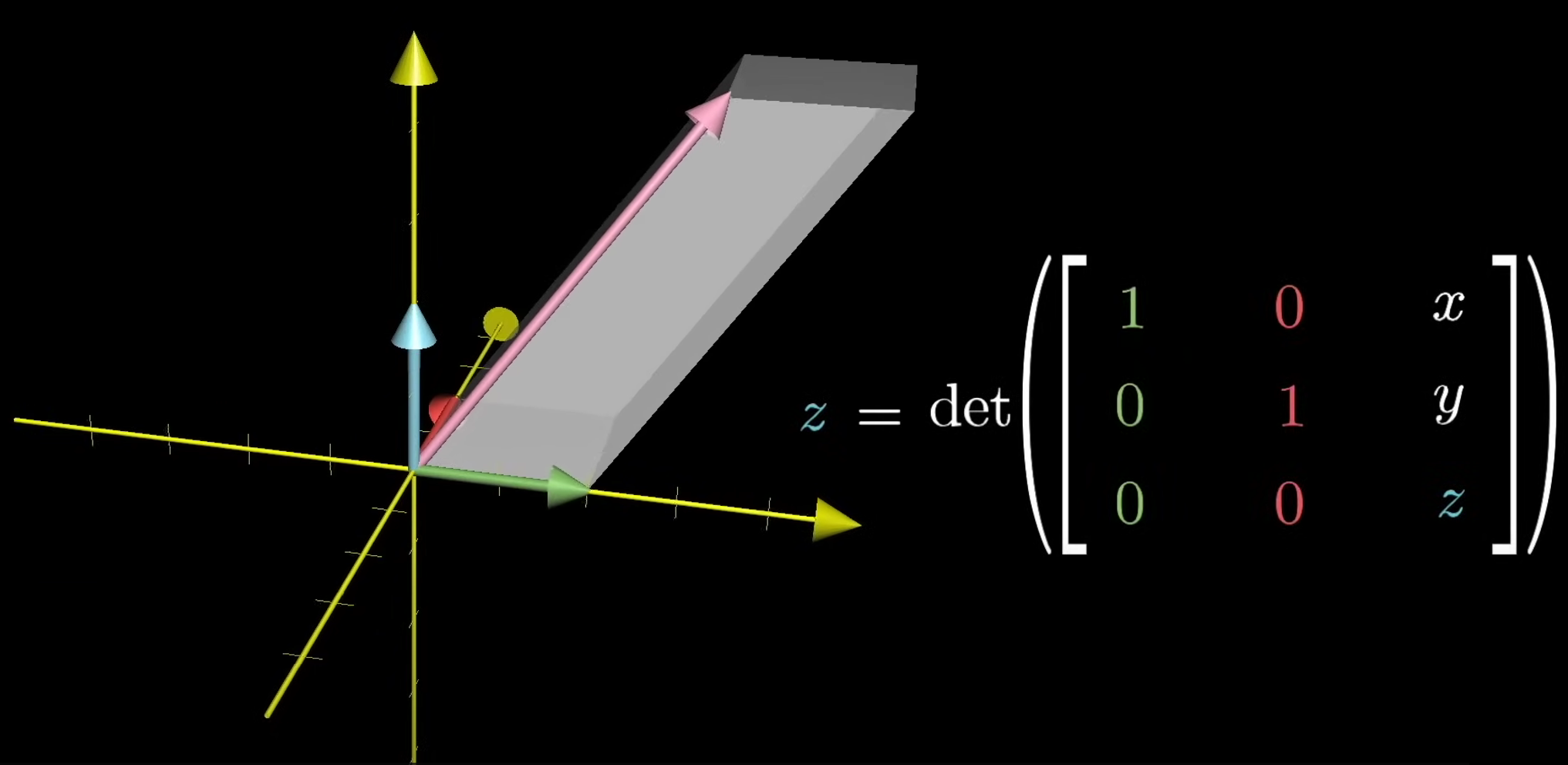
Then apply with a linear transformation:![]()
The question becomes
$$
\begin{bmatrix}
\color{green}a_{11} & \color{red}a_{12} & \color{blue}a_{13} \\
\color{green}a_{21} & \color{red}a_{22} & \color{blue}a_{23} \\
\color{green}a_{31} & \color{red}a_{32} & \color{blue}a_{33}
\end{bmatrix}
\begin{bmatrix} x \\ y \\ z \end{bmatrix}
=
\begin{bmatrix} b_1 \\ b_2 \\ b_3 \end{bmatrix}
$$
Then we can solve for z:
$$
\begin{equation}
z = \cfrac{\text{Volume of Parallelepiped}}{|A|} =
\cfrac{
\begin{vmatrix}
\color{green}a_{11} & \color{red}a_{12} & b_1 \\
\color{green}a_{21} & \color{red}a_{22} & b_2 \\
\color{green}a_{31} & \color{red}a_{32} & b_3
\end{vmatrix}
}{
\begin{vmatrix}
\color{green}a_{11} & \color{red}a_{12} & \color{blue}a_{13} \\
\color{green}a_{21} & \color{red}a_{22} & \color{blue}a_{23} \\
\color{green}a_{31} & \color{red}a_{32} & \color{blue}a_{33}
\end{vmatrix}
}
\end{equation}
$$
Similarly,
$$
\begin{equation}
x =
\cfrac{
\begin{vmatrix}
b_1 & \color{red}a_{12} & \color{blue}a_{13} \\
b_2 & \color{red}a_{22} & \color{blue}a_{23} \\
b_3 & \color{red}a_{32} & \color{blue}a_{33}
\end{vmatrix}
}{
\begin{vmatrix}
\color{green}a_{11} & \color{red}a_{12} & \color{blue}a_{13} \\
\color{green}a_{21} & \color{red}a_{22} & \color{blue}a_{23} \\
\color{green}a_{31} & \color{red}a_{32} & \color{blue}a_{33}
\end{vmatrix}
}
,
y =
\cfrac{
\begin{vmatrix}
\color{green}a_{11} & b_1 & \color{blue}a_{13} \\
\color{green}a_{21} & b_2 & \color{blue}a_{23} \\
\color{green}a_{31} & b_3 & \color{blue}a_{33}
\end{vmatrix}
}{
\begin{vmatrix}
\color{green}a_{11} & \color{red}a_{12} & \color{blue}a_{13} \\
\color{green}a_{21} & \color{red}a_{22} & \color{blue}a_{23} \\
\color{green}a_{31} & \color{red}a_{32} & \color{blue}a_{33}
\end{vmatrix}
}
\end{equation}
$$
8. Change of Basis
If there is a vector sitting in 2-D space, we have a standard way to describe it with coordinate: $\begin{bmatrix} x \\ y \end{bmatrix}$. It means the vector is $x\hat i + y\hat j$.
What if we used different basis vectors?
For example, if there is a world using basis vector as $\vec b_1 = \begin{bmatrix} 2 \\ 1 \end{bmatrix}$ and $\vec b_2 = \begin{bmatrix} -1 \\ 1 \end{bmatrix}$, and there is a vector using their world language: $\begin{bmatrix} -1 \\ 2 \end{bmatrix}$
We can translate the vector into our language as $\vec v=(-1)\vec b_1+2\vec b_2=-1\begin{bmatrix} 2 \\ 1 \end{bmatrix}+2 \begin{bmatrix} -1 \\ 1 \end{bmatrix} = \begin{bmatrix} -4 \\ 1 \end{bmatrix}$
Is it a deja vu? We can use a matrix to describe it:
$$
\begin{equation}
\underbrace{\begin{bmatrix} -4 \\ 1 \end{bmatrix}}_{\underset{\scriptsize\textstyle\text{language}}{\text{vector in our}}}
=
\overbrace{\begin{bmatrix} 2 & -1 \\ 1 & 1 \end{bmatrix}}^{\text{translation}}
\underbrace{\begin{bmatrix} -1 \\ 2 \end{bmatrix}}_{\underset{\scriptsize\textstyle\text{language}}{\underset{\scriptsize\textstyle\text{their}}{\text{vector in}}}}
\end{equation}
$$
If we want to translate our language to their language, you just multiply an inverse A:
\begin{equation}
\underbrace{\begin{bmatrix} -1 \\ 2 \end{bmatrix}}_{\underset{\scriptsize\textstyle\text{language}}{\underset{\scriptsize\textstyle\text{their}}{\text{vector in}}}}
=
\overbrace{\begin{bmatrix} \frac{1}{3} & \frac{1}{3} \\ -\frac{1}{3} & \frac{2}{3} \end{bmatrix}}^{A^{-1}}
\underbrace{\begin{bmatrix} -4 \\ 1 \end{bmatrix}}_{\underset{\scriptsize\textstyle\text{language}}{\text{vector in our}}}
\end{equation}
However, vectors are not the only thing in coordinates.
Consider some linear transformation, like a 90-degree counterclockwise rotation. The matrix in our language is $\begin{bmatrix}0 & -1 \\ 1 & 0 \end{bmatrix}$.
How to translate the same 90-degree counterclockwise rotation in their language? Multiplying the matrix with the translation matrix mentioned above is not right. Because the columns of the rotation matrix still represent our basis, not theirs. So multiplying the matrix with the translation matrix outputs a wrong matrix which is not really 90-degree counterclockwise rotation.
To translate the matrix, we can start with a random vector in their language: $\vec v$
In order to describe the rotation, we firstly translate it into our language:
$$
\overbrace{
\underbrace{\begin{bmatrix} 2 & -1 \\ 1 & 1 \end{bmatrix}}_{\text{translation}}
\vec v
}^{\text{vector in our language}}
$$
Then apply the transformation matrix by multiplying it on the left
$$
\overbrace{
\underbrace{\begin{bmatrix} 0 & -1 \\ 1 & 0 \end{bmatrix}}_{\text{Rotation}}
\begin{bmatrix} 2 & -1 \\ 1 & 1 \end{bmatrix}
\vec v
}^{\text{vector after transformation in our language}}
$$
Last step, apply the inverse matrix change of basis matrix, multiplied it on the left, to translate it back into their language.
$$
\overbrace{
\underbrace{\begin{bmatrix} 2 & -1 \\ 1 & 1 \end{bmatrix}^{-1}}_{\text{Translate back}}
\begin{bmatrix} 0 & -1 \\ 1 & 0 \end{bmatrix}
\begin{bmatrix} 2 & -1 \\ 1 & 1 \end{bmatrix}
\vec v
}^{\text{vector after transformation in their language}}
$$
So the transformation matrix in their language is $
\begin{bmatrix} 2 & -1 \\ 1 & 1 \end{bmatrix}^{-1}
\begin{bmatrix} 0 & -1 \\ 1 & 0 \end{bmatrix}
\begin{bmatrix} 2 & -1 \\ 1 & 1 \end{bmatrix}
=
\begin{bmatrix} \frac{1}{3} & -\frac{2}{3} \\ \frac{5}{3} & -\frac{1}{3} \end{bmatrix}
$
An expression like $A^{-1}MA$ suggests a mathematical sort of empathy, that middle matrix $M$ represents a transformation of some kind as you see it, and the outer two matrices $A^{-1}$ and $A$ represent the empathy, the shift in perspective. And the full matrix product represents that same transformation but someone else sees it.
9. Eigenvectors, Eigenvalues and Diagonalization
9.1 What is Eigenvectors and Eigenvalues
Consider there is a linear transformation and a vector and think of the span of the vector. Most vectors are going to get knocked off their span during the transformation.![]()
But some vectors do remain on their own span.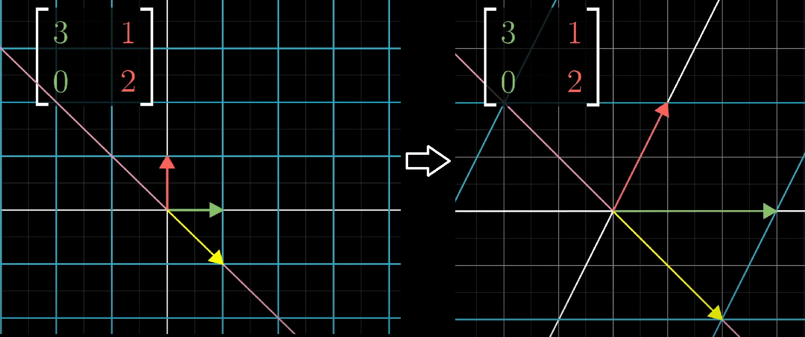
In this case, the vector is scaled by some number. These vectors are called eigenvectors. And the factors by which it’s scaled are called eigenvalues. In addition, there may be more than one line of eigenvectors exists after transformation.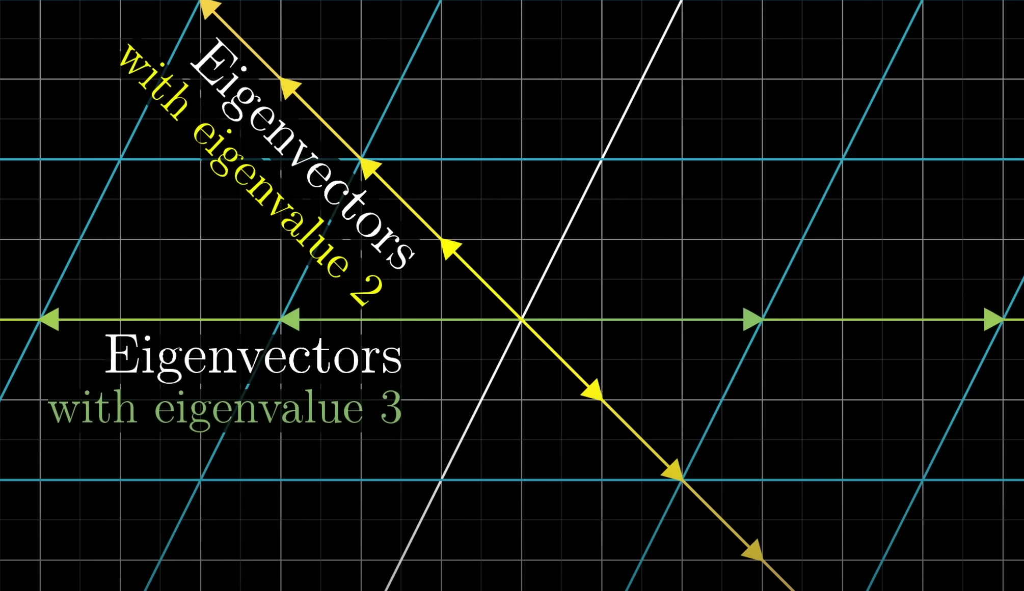
The eigenvalues can also be negative.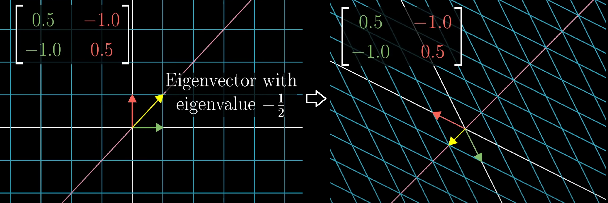
So the eigenvectors can be used for what?
Consider some 3-D rotation. If you can find an eigenvector for that rotation, what you have found is the axis of rotation.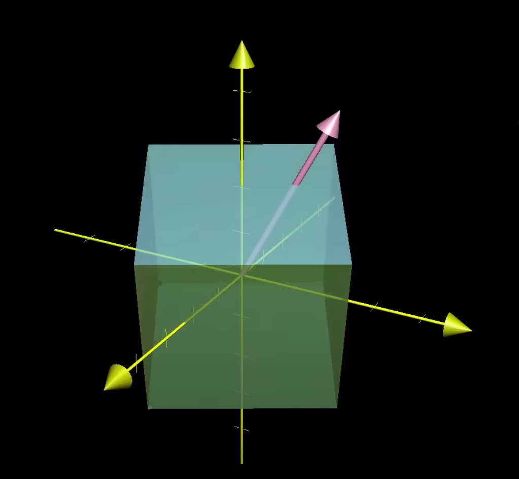
In this case, the eigenvalue would have to be 1, since rotations never stretch or squish anything.
The eigenvectors looks like:
$$
A\vec v = \lambda\vec v
$$
A is the matrix representing some transformation, with $\vec v$ as the eigenvector, and $\lambda$ is a number, namely the corresponding eigenvalue.
There are some properties of eigenvalues:
- $A$ and $A^T$ have the same eigenvalues.
- If $\lambda$ is an eigenvalue of $A$, then $\lambda^2$ is a eigenvalue of $A^2$.
9.2 How to Get Eigenvectors and Eigenvalues
The eigenvectors are the vectors scaled by some number after transformation like $\lambda\vec v$. So the transformation matrix of the vector can be
$$
\begin{bmatrix}
\lambda & 0 & 0 \\
0 & \lambda & 0 \\
0 & 0 & \lambda
\end{bmatrix}
=
\lambda
\begin{bmatrix}
1 & 0 & 0 \\
0 & 1 & 0 \\
0 & 0 & 1
\end{bmatrix}
=
\lambda I
$$
So $A\vec v = \lambda\vec v$ can be $A\vec v = (\lambda I)\vec v$. With both sides looking like matrix-vector multiplication, we can subtract off that right-hand side and factor out the $\vec v$.
$$
A\vec v - (\lambda I)\vec v = (A - \lambda I)\vec v = 0
$$
So we have a new matrix $A - \lambda I$. If $A=\begin{bmatrix} 3 & 1 & 4 \\ 1 & 5 & 9 \\ 2 & 6 & 5 \end{bmatrix}$, then the new matrix can be written as:
$$
\begin{bmatrix}
3-\lambda & 1 & 4 \\
1 & 5-\lambda & 9 \\
2 & 6 & 5-\lambda
\end{bmatrix}
$$
What we want is a non-zero eigenvector, so the new matrix $A - \lambda I$ make the vector $\vec v$ zero.
The only way that’s possible for the product of matrix with a non-zero vector to become zero is if the transformation associated with that matrix squishes space into a lower dimension. So the determinant of that matrix must be zero.
$$
det(A-\lambda I) =
\begin{vmatrix}
3-\lambda & 1 & 4 \\
1 & 5-\lambda & 9 \\
2 & 6 & 5-\lambda
\end{vmatrix}
= 0
$$
So we have to find some $\lambda$ to make the determinant of that matrix zero.
Take a 2x2 matrix for example:
$$
det(A-\lambda I) =
\begin{vmatrix}
2-\lambda & 2 \\
1 & 3-\lambda
\end{vmatrix}
= (2-\lambda)(3-\lambda) -2 = 0
$$
In this case, the only possible eigenvalues are $\lambda = 1$ and $\lambda = 4$.
Then plug in each $\lambda$ to the matrix and solve for which vectors this diagonally altered matrix sends to zero.
$$
\begin{align*}
\text{for }\lambda\text{=1}:\qquad & \\
& \begin{bmatrix} 2-1 & 2 \\ 1 & 3-1 \end{bmatrix}
\begin{bmatrix} x \\ y \end{bmatrix}
= \begin{bmatrix} 0 \\ 0 \end{bmatrix} \\
& x = -2y \\
\text{for }\lambda\text{=4}:\qquad & \\
& \begin{bmatrix} 2-4 & 2 \\ 1 & 3-4 \end{bmatrix}
\begin{bmatrix} x \\ y \end{bmatrix}
= \begin{bmatrix} 0 \\ 0 \end{bmatrix} \\
& x = y
\end{align*}
$$
Some transformations do not have eigenvectors.
For example, for a rotation matrix $\begin{bmatrix} 0 & -1 \\ 1 & 0 \end{bmatrix}$, it has no eigenvectors, since it rotates every vectors off of its own span.
If you try computing the eigenvalues of a rotation like this:
$$
\begin{align*}
det(A-\lambda I) =
\begin{vmatrix}
-\lambda & -1 \\
1 & -\lambda
\end{vmatrix}
&= (-\lambda)(-\lambda)-(-1)1 \\
&= \lambda ^2 + 1 = 0 \\
\lambda = i \text{ or } \lambda = -i
\end{align*}
$$
The fact that there are no real number solutions indicates that there are no eigenvectors.
The eigenvalues which are complex numbers correspond to some kind of rotation in the transformation. But it’s beyond the essence of linear transformation. If you are interested in it, you can google it.
Note that a single eigenvalue can have more than just a line full of eigenvectors.
For example, there is a matrix that scales everything by 2: $A=\begin{bmatrix} 2 & 0 \\ 0 & 2 \end{bmatrix}$.
The only eigenvalue is 2, but every vector in the plane gets to be an eigenvector with that eigenvalue.
9.3 A Quick Trick for Computing Eigenvalues
There are three facts we have to know:
- The trace $tr(\begin{bmatrix} \boxed{a} & b \\ c & \boxed{d} \end{bmatrix}) = a + d = \lambda_1 + \lambda_2=2m$, so $\begin{equation}m=\cfrac{a+d}{2}\end{equation}$ is the mean of the trace.
- $det(A)=\begin{bmatrix} a & b \\ c & d \end{bmatrix}=ad-bc=\lambda_1 \lambda_2=p$.
- $\lambda_1,\ \lambda_2=m\pm\sqrt{m^2-p}$.
This trick can help you get the eigenvalues quickly with simple matrices.
Proof:
$$
\begin{align*}
det(A-\lambda I) =
\begin{vmatrix}
a-\lambda & b \\
c & d-\lambda
\end{vmatrix}
&= (a-\lambda)(d-\lambda) -bc \\
&= \lambda^2 - (a+d)\lambda + (ad-bc) \\
&= \lambda^2 - tr(A)\lambda + det(A) \\
&= 0 \\
\text{Solve the quadratic equation: }\qquad \lambda &= \cfrac{tr(A) \pm \sqrt{(-tr(A))^2 - 4det(A)}}{2} \\
&= \cfrac{tr(A)}{2} \pm \sqrt{\cfrac{(tr(A))^2}{4} - \cfrac{4det(A)}{4}} \\
&= \cfrac{tr(A)}{2} \pm \sqrt{(\cfrac{tr(A)}{2})^2 - det(A)} \\
\text{Let }\quad m=\cfrac{tr(A)}{2},\ p=det(A), \\
\text{then }\quad \lambda = m \pm \sqrt{m^2 - p}
\end{align*}
$$
9.4 Eigenbasis and Diagonalization
Think about the diagonal matrix, which has zeros everywhere other than the diagonal:
$$
\begin{bmatrix}
-5 & 0 & 0 & 0 \\
0 & -2 & 0 & 0 \\
0 & 0 & -4 & 0 \\
0 & 0 & 0 & 4
\end{bmatrix}
$$
And the way to interpret it is that all the basis vectors are eigenvectors, with the diagonal entries of this matrix being their eigenvalues.
$$
\begin{align*}
& det(A-\lambda I) = (-5-\lambda)(-2-\lambda)(-4-\lambda)(4-\lambda)=0 \\
& \begin{cases} \lambda=-5 \\ \lambda=-2 \\ \lambda=-4 \\ \lambda=4 \end{cases}
\end{align*}
$$
There are a lot of things that make diagonal matrices much nicer to work with.
For example, if you multiply the matrix itself several times:
$$
\underbrace{
\begin{bmatrix} 3 & 0 \\ 0 & 2 \end{bmatrix} \cdots
\begin{bmatrix} 3 & 0 \\ 0 & 2 \end{bmatrix} \begin{bmatrix} 3 & 0 \\ 0 & 2 \end{bmatrix}
}_{\text{100 times}}
\begin{bmatrix} x \\ y \end{bmatrix}
=
\begin{bmatrix} 3^{100} & 0 \\ 0 & 2^{100} \end{bmatrix}
\begin{bmatrix} x \\ y \end{bmatrix}
$$
In contract, try computing the 100th power of a non-diagonal matrix is a nightmare.
However, changing the basis can be useful to solve this problem by hand quickly.
For example, for a matrix $B=\begin{bmatrix} 3 & 1 \\ 0 & 2 \end{bmatrix}$, the eigenvalues are $\lambda=\color{red}2$ and $\lambda=\color{red}3$, and the lines of eigenvectors are $x=-y$ and $y=0$. So we can choose the basis vectors $\begin{bmatrix} 1 \\ 0 \end{bmatrix}$ and $\begin{bmatrix} -1 \\ 1 \end{bmatrix}$.
Then make those coordinates of matrix, known as the change of basis matrix: $\begin{bmatrix} 1 & -1 \\ 0 & 1 \end{bmatrix}$.
Then you can write as $\Lambda=P^{-1}BP$ representing the same transformation, but from the perspective of the new basis. And this new matrix is guaranteed to be diagonal with its corresponding eigenvalues down that diagonal. This is because it represents working in a coordinate system where what happens to the basis vectors is that they get scaled during the transformation.
$$
\begin{bmatrix} 1 & -1 \\ 0 & 1 \end{bmatrix}^{-1}
\begin{bmatrix} 3 & 1 \\ 0 & 2 \end{bmatrix}
\begin{bmatrix} 1 & -1 \\ 0 & 1 \end{bmatrix}
=
\begin{bmatrix} \color{red}3 & 0 \\ 0 & \color{red}2 \end{bmatrix}
$$
The method to let a matrix diagonal is called diagonalization.
A set of basis vectors which are also eigenvectors is called an eigenbasis.
So to compute the 100th power, you change to an eigenbasis, then compute the 100th power in that system, then convert back to our standard system.
$$
B^k = (P\Lambda P^{-1})^k = P\Lambda^{k}P^{-1} =
\begin{bmatrix} 1 & -1 \\ 0 & 1 \end{bmatrix}
\begin{bmatrix} 3^k & 0 \\ 0 & 2^k \end{bmatrix}
\begin{bmatrix} 1 & -1 \\ 0 & 1 \end{bmatrix}^{-1}
$$
Notice that not all matrices can become diagonal by changing basis. Some matrices do not have enough eigenvectors to span the full space.
When is the matrix diagonalizable?
The matrix is diagonalizable when all the eigenvalues $\lambda$ is different.
Because when there are repeated eigenvalues, for example $\begin{bmatrix} 3 & 1 \\ 0 & 3 \end{bmatrix}$ has eigenvalues $\lambda_1=\lambda_2=3$, which is called degenerate matrix, we may not have enough independent vectors. So the example matrix cannot be diagonalized.
10. Abstract Vector Spaces
10.1 What is Vector Space
What is vector?
We describe vector as an arrow with several numbers, i.e. coordinate. However, vector is more than the vector we described before.
Vector space is an abstract concept. Why calling it space?
We can make an analogy between vectors and functions.
When we add two functions $f(x)$ and $g(x)$ together, the output is the sum of the outputs of f and g when you evaluate them each at that same input.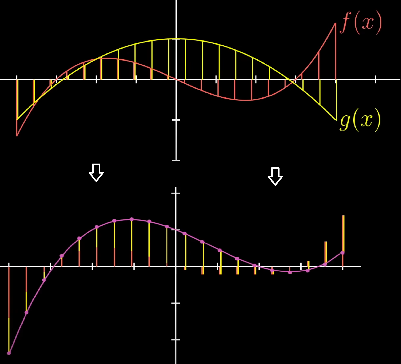
It’s similar to adding vectors coordinate by coordinate
$$
\begin{bmatrix} a_1 \\ a_2 \\ a_3 \\ \vdots \end{bmatrix} +
\begin{bmatrix} b_1 \\ b_2 \\ b_3 \\ \vdots \end{bmatrix} =
\begin{bmatrix} a_1 + b_1 \\ a_2 + b_2 \\ a_3 + b_3 \\ \vdots \end{bmatrix}
$$
Similarly, scaling a function by a real number just scales all the outputs by that number.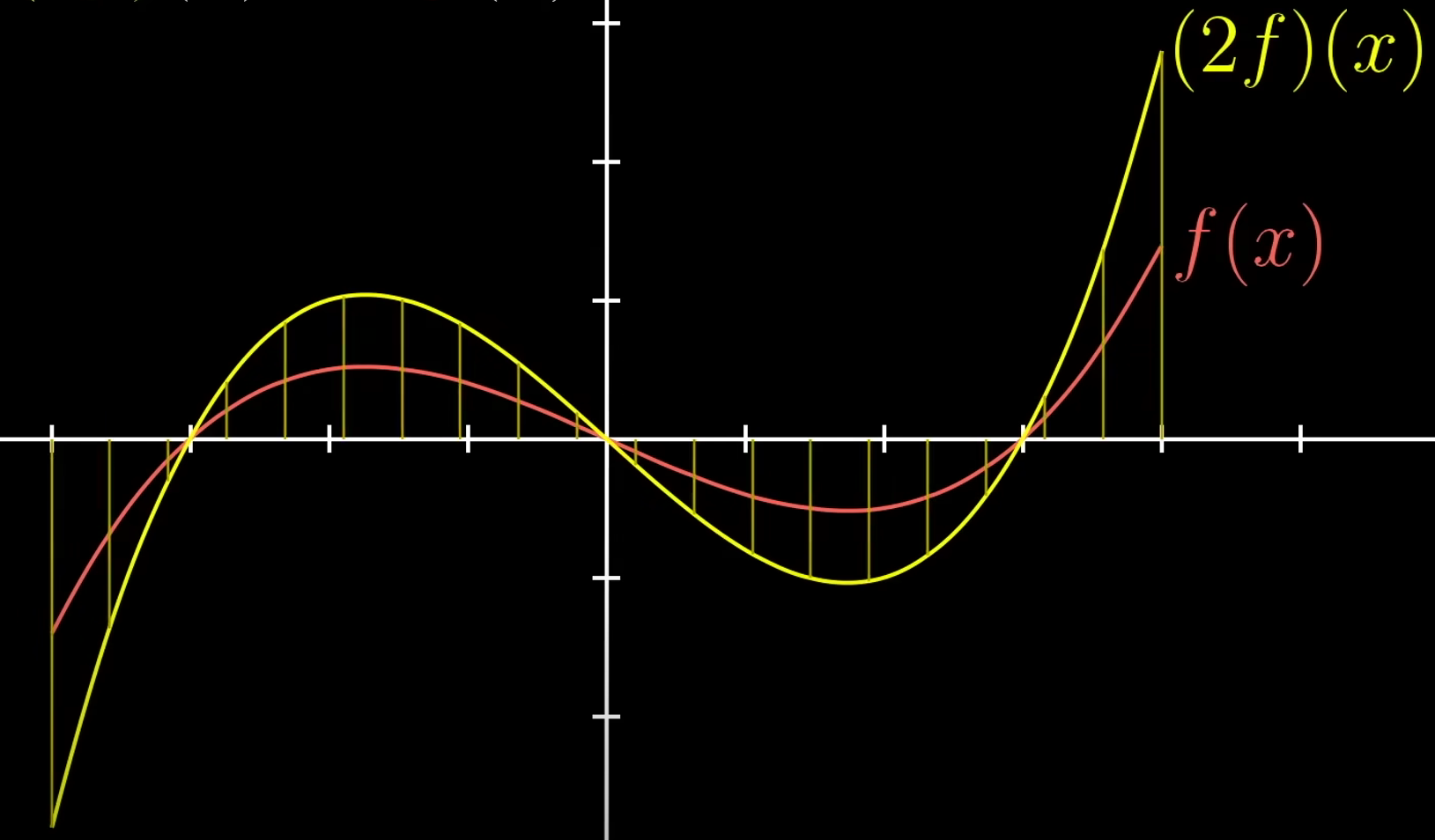
It’s analogous to scale a vector coordinate by coordinate.
$$
k\begin{bmatrix} a_1 \\ a_2 \\ a_3 \\ \vdots \end{bmatrix} =
\begin{bmatrix} k a_1 \\ k a_2 \\ k a_3 \\ \vdots \end{bmatrix}
$$
When we talk in linear algebra language, the function should be linear.
Formal definition of linearity:
- Additivity: $L(\vec v + \vec w) = L(\vec v) + L(\vec w)$
- Scaling: $L(c\vec v) = cL(\vec v)$
Additivity means that if you add two vector $\vec v$ and $\vec w$, then apply a transformation to their sum, you get the same result as if you added the transformed versions of $\vec v$ and $\vec w$:
$$
A(\vec v + \vec w)=A\vec v + A\vec w
$$
The scaling property is that when you scale a vector by some number, then apply the transformation, you get the same ultimate vector as if you scaled the transformed version of $\vec v$ by that same amount.
$$
A(c\vec v)=c(A\vec v)
$$
Linear transformations preserve addition and scalar multiplication.
There are a lot of useful tools in linear algebra we can use, such as linear transformation, null space, dot products, eigenvectors and so forth, to apply them to functions to solve the problem.
For example, we can use linear transformation to describe the derivative.
Derivative is additive and has the scaling property:
- $\begin{equation} \cfrac{\mathrm{d}}{\mathrm{d}x}(x^3 + x^2) = \cfrac{\mathrm{d}}{\mathrm{d}x} x^3 + \cfrac{\mathrm{d}}{\mathrm{d}x} x^2 \end{equation}$
- $\begin{equation} \cfrac{\mathrm{d}}{\mathrm{d}x}(4x^3) = 4 \cdot \cfrac{\mathrm{d}}{\mathrm{d}x}(x^3) \end{equation}$
Then let’s describe the derivative with a matrix(Limiting the space to all polynomials).
The first thing we need to do is give coordinates to this space.
Since polynomials are already written down as the sum of scaled powers of the variable $x$, it’s natural to choose powers of $x$ as the basis function
$$
\begin{gather}
\text{Basis Functions} \\
b_0(x)=1 \\
b_1(x)=x \\
b_2(x)=x^2 \\
b_3(x)=x^3 \\
\vdots
\end{gather}
$$
Then describe the coefficients as the coordinates of the vector:
$$
a_0 + a_1 x + a_2 x^2 + a_3 x^3 + \cdots + a_n x^n =
\begin{bmatrix} a_0 \\ a_1 \\ a_2 \\ a_3 \\ \vdots \\ a_n \end{bmatrix}
$$
For example
$$
5 + 3x + x^2 = \begin{bmatrix} 5 \\ 3 \\ 1 \\ 0 \\ 0 \\ \vdots \end{bmatrix}
$$
In this coordinate system, the derivative is described with this matrix:
$$
\begin{equation}
\cfrac{\mathrm{d}}{\mathrm{d}x}=
\begin{bmatrix}
0 & 1 & 0 & 0 & \cdots \\
0 & 0 & 2 & 0 & \cdots \\
0 & 0 & 0 & 3 & \cdots \\
0 & 0 & 0 & 0 & \cdots \\
\vdots & \vdots & \vdots & \vdots & \ddots
\end{bmatrix}
\end{equation}
$$
If we multiply a vector by that matrix, it represents the derivative.
For example
$$
\begin{gather}
\cfrac{\mathrm{d}}{\mathrm{d}x}(5 + 4x + 5x^2 + x^3)= \color{green}4 \color{black}+ \color{red}10\color{black}x + \color{blue}3\color{black}x^2 \\
\begin{bmatrix}
0 & 1 & 0 & 0 & \cdots \\
0 & 0 & 2 & 0 & \cdots \\
0 & 0 & 0 & 3 & \cdots \\
0 & 0 & 0 & 0 & \cdots \\
\vdots & \vdots & \vdots & \vdots & \ddots
\end{bmatrix}
\begin{bmatrix} 5 \\ 4 \\ 5 \\ 1 \\ 0 \\ \vdots \end{bmatrix}
=
\begin{bmatrix} \color{green}4 \\ \color{red}10 \\ \color{blue}3 \\ 0 \\ 0 \\ \vdots \end{bmatrix}
\end{gather}
$$
What makes it possible is that the derivative is linear.
These sets of vectorish things, like arrows or lists of numbers or functions, are called vector spaces.
So you can use the linear algebra as a tool to solve the problem like this.
You establish a list of rules that vector addition and scaling have to abide by. These rules are called axioms. In modern theory of linear algebra, there are eight axioms that any vector space must satisfy:
- $\vec u + (\vec v + \vec w) = (\vec u + \vec v) + \vec w$
- $\vec v + \vec w = \vec w + \vec v$
- $\vec 0 + \vec v = \vec v \text{ for all }\vec v$
- $\vec v + (-\vec v) = 0 \text{ for all }\vec v$
- $a(b\vec v)=(ab)\vec v$
- $1\vec v = \vec v$
- $a(\vec v + \vec w) = a\vec v + a\vec w$
- $(a+b)\vec v = a\vec v + b\vec v$
These axioms are not rules of nature, but an interface. These axioms are like a checklist of things that they need to verify about their definitions before they can start applying the results of linear algebra.
10.2 Subspaces
We use $\mathbb{R}^n$ to represent n real numbers or n-dim real vectors. For example, $\mathbb{R}^2$ represents 2 real numbers or 2-D real vectors.
Vector space requirements: if $\vec v$ and $\vec w$ are in the space, then $\vec v + \vec w$, $k\vec v$ and the linear combination $a\vec v + b\vec w$ are also in the space.
So a plane or a line through the origin is the subspace of $\mathbb{R}^3$.
Let P as a plane through the origin and L as a line through the origin.
For $P \cup L$, if the line is in the plane, then $P \cup L = P$ is a subspace of $\mathbb{R}^3$. However, if the line is NOT in the plane, then $P \cup L$ is not a subspace of $\mathbb{R}^3$ because it doesn’t fit the requirements.
For $P \cap L$, if the line is in the plane, then $P \cap L = L$ is a subspace of $\mathbb{R}^3$. If the line is not in the plane, the $P \cap L$ is the origin, meaning there is only a zero-vector in the space. In this case, $P \cap L$ is still a subspace of $\mathbb{R}^3$.
For a matrix like a 4x3 matrix, it’s a column space of $\mathbb{R}^4$. It’s all linear combinations of columns.
Null space is all the solutions of $Ax=0$.
For example,
$$
Ax =
\begin{bmatrix}
1 & 1 & 2 \\
2 & 1 & 3 \\
3 & 1 & 4 \\
4 & 1 & 5
\end{bmatrix}
\begin{bmatrix} x_1 \\ x_2 \\ x_3 \end{bmatrix}
=
\begin{bmatrix} 0 \\ 0 \\ 0 \\ 0 \end{bmatrix}
$$
The solutions x can be $\begin{bmatrix} c \\ c \\ -c \end{bmatrix}$, c is any number.
The solutions to $Ax=0$ always give a nullspace. So if $Av=0$ and $Aw=0$, then $A(v+w)=0$. If v and w are nullspaces, then $v+w$ is a nullspace.
Here is an example question:
Find the dimension of the vector space spanned by the vectors below and find a basis for that space.
$$
\begin{gather}
(1,1,-2,0,-1) \\
(1,2,0,-4,1) \\
(0,1,3,-3,2) \\
(2,3,0,-2,0)
\end{gather}
$$
To find a basis for the space, we just pack the vectors in a matrix and then do elimination.
$$
\begin{equation}
\begin{bmatrix}
1 & 1 & -2 & 0 & -1 \\
1 & 2 & 0 & -4 & 1 \\
0 & 1 & 3 & -3 & 2 \\
2 & 3 & 0 & -2 & 0
\end{bmatrix}
\xrightarrow{eliminate}
\begin{bmatrix}
1 & 1 & -2 & 0 & -1 \\
0 & 1 & 2 & -4 & 2 \\
0 & 0 & 1 & 1 & 0 \\
0 & 0 & 0 & 0 & 0
\end{bmatrix}
\end{equation}
$$
After elimination, we found three pivot of the matrix, and the last vector is useless.
So there are three basis vectors: $\begin{bmatrix} 1 \\ 1 \\ -2 \\ 0 \\ -1 \end{bmatrix}$, $\begin{bmatrix} 0 \\ 1 \\ 2 \\ -4 \\ 2 \end{bmatrix}$ and $\begin{bmatrix} 0 \\ 0 \\ 1 \\ 1 \\ 0 \end{bmatrix}$.
The dimension is three. There are 5 dimensions in each vector, so why not 5?
Imagine there is a line in a 3-dimensional space, How many dimension does the line have? Absolutely only one. If there are three vectors in 3-D space but just span a 2-dimensional plane, then the vector space has only 2 dimensions. So if there are four vectors in 5-dimensional space but just span a 3-dimensional space, the vector space has only 3 dimensions.
In this example, we put vectors in the rows of the matrix. What if we put them in columns? That also works.
$$
\begin{equation}
\begin{bmatrix}
1 & 1 & 0 & 2 \\
1 & 2 & 1 & 3 \\
-2 & 0 & 3 & 0 \\
0 & -4 & -3 & -2 \\
-1 & 1 & 2 & 0
\end{bmatrix}
\xrightarrow{eliminate}
\begin{bmatrix}
1 & 1 & 0 & 2 \\
0 & 1 & 1 & 1 \\
0 & 0 & 1 & 2 \\
0 & 0 & 0 & 0 \\
0 & 0 & 0 & 0
\end{bmatrix}
\end{equation}
$$
Obviously there are 3 dimensions.
But we cannot pick the first three columns of vectors in eliminated matrix as basis vectors. Because when we do elimination, we change the column space. So what we need to do is to pick three column vectors in the same position of columns in the original matrix.
So the basis vectors are $\begin{bmatrix} 1 \\ 1 \\ -2 \\ 0 \\ -1 \end{bmatrix}$, $\begin{bmatrix} 1 \\ 2 \\ 0 \\ -4 \\ 1 \end{bmatrix}$ and $\begin{bmatrix} 0 \\ 1 \\ 3 \\ -3 \\ 2 \end{bmatrix}$.
10.3 Four Fundamental Subspaces
Suppose A is a mxn matrix.
- The column space $C(A)$ in $\mathbb{R}^m$. $dim(C(A))=rank(A)$.
- The null space $N(A)$ in $\mathbb{R}^n$. $dim(N(A))=n-rank(A)$.
- The row space, can be written as $C(A^T)$ in $\mathbb{R}^n$. $dim(C(A^T))=rank(A)$.
- The transpose of null space $N(A^T)$ in $\mathbb{R}^m$, can be called as the left nullspace of A. $dim(N(A^T))=m-rank(A)$.
When we do an elimination, like $A \xrightarrow{eliminate} R$, the column space has changed. So $A \ne R$. However, the row space haven’t been affected.
For the left nullspace, $A^T y=0$
$$
\begin{bmatrix}
\quad & \quad & \quad & \quad \\
\quad & \quad & \quad & \quad \\
\quad & \quad & \quad & \quad
\end{bmatrix}
\begin{bmatrix}
\quad \\ \quad \\ \quad \\ \quad
\end{bmatrix}
=
\begin{bmatrix}
0 \\ 0 \\ \vdots \\ 0
\end{bmatrix}
$$
Take a transpose to get $(A^T y)^T = y^T (A^T)^T = y^T A = 0^T$:
$$
\begin{bmatrix}
\quad & \quad & \quad & \quad
\end{bmatrix}
\begin{bmatrix}
\quad & \quad & \quad \\
\quad & \quad & \quad \\
\quad & \quad & \quad \\
\quad & \quad & \quad
\end{bmatrix}
=
\begin{bmatrix}
0 & 0 & \cdots & 0
\end{bmatrix}
$$
To find the basis for $N(A^T)$, we have to find which basis change the rwo of $A$ to 0.
For example,
$$
B = LU =
\begin{bmatrix}
1 & & \\
2 & 1 & \\
-1 & 0 & 1
\end{bmatrix}
\begin{bmatrix}
5 & 0 & 3 \\
0 & 1 & 1 \\
0 & 0 & 0
\end{bmatrix}
$$
We need to get $L^{-1}B=U$:
$$
\begin{bmatrix}
1 & & \\
-2 & 1 & \\
\color{red}1 & \color{red}0 & \color{red}1
\end{bmatrix}
B =
\begin{bmatrix}
5 & 0 & 3 \\
0 & 1 & 1 \\
\color{red}0 & \color{red}0 & \color{red}0
\end{bmatrix}
$$
The third row of $L^{-1}$ make the third row of B 0. So there is one basis of $N(A^T)$: $\begin{bmatrix} 1 \\ 0 \\ 1 \end{bmatrix}$.
10.4 Matrix Spaces
Take 3x3 matrix $M$ as example.
Basis for $M$:
$$
\begin{bmatrix} 1 & 0 & 0 \\ 0 & 0 & 0 \\ 0 & 0 & 0 \end{bmatrix},
\begin{bmatrix} 0 & 1 & 0 \\ 0 & 0 & 0 \\ 0 & 0 & 0 \end{bmatrix},
\begin{bmatrix} 0 & 0 & 1 \\ 0 & 0 & 0 \\ 0 & 0 & 0 \end{bmatrix},
\cdots
\begin{bmatrix} 0 & 0 & 0 \\ 0 & 0 & 0 \\ 0 & 0 & 1 \end{bmatrix},
$$
The dimension of the matrix is 9.
We can get any 3x3 matrix by the linear combination of basis matrices.
$$
A =
c_1 \begin{bmatrix} 1 & 0 & 0 \\ 0 & 0 & 0 \\ 0 & 0 & 0 \end{bmatrix} +
c_2 \begin{bmatrix} 0 & 1 & 0 \\ 0 & 0 & 0 \\ 0 & 0 & 0 \end{bmatrix} +
\cdots +
c_9 \begin{bmatrix} 0 & 0 & 0 \\ 0 & 0 & 0 \\ 0 & 0 & 1 \end{bmatrix}
$$
Then the subspace of $M$.
Take symmetric matrices space $S$ as an example, there are 3 diagonal positions and 3 symmetric numbers. So $dim(S)=6$.
$$
\begin{align}
\begin{bmatrix}
c_1\color{red}a & c_4\color{blue}x & c_5\color{green}y \\
c_4\color{blue}x & c_2\color{red}b & c_6\color{purple}z \\
c_5\color{green}y & c_6\color{purple}z & c_3\color{red}c
\end{bmatrix}
=&
c_1\begin{bmatrix} \color{red}a & 0 & 0 \\ 0 & 0 & 0 \\ 0 & 0 & 0 \end{bmatrix} +
c_2\begin{bmatrix} 0 & 0 & 0 \\ 0 & \color{red}b & 0 \\ 0 & 0 & 0 \end{bmatrix} +
c_3\begin{bmatrix} 0 & 0 & 0 \\ 0 & 0 & 0 \\ 0 & 0 & \color{red}c \end{bmatrix} + \\
&
c_4\begin{bmatrix} 0 & \color{blue}x & 0 \\ \color{blue}x & 0 & 0 \\ 0 & 0 & 0 \end{bmatrix} +
c_5\begin{bmatrix} 0 & 0 & \color{green}y \\ 0 & 0 & 0 \\ \color{green}y & 0 & 0 \end{bmatrix} +
c_6\begin{bmatrix} 0 & 0 & 0 \\ 0 & 0 & \color{purple}z \\ 0 & \color{purple}z & 0 \end{bmatrix}
\end{align}
$$
Take upper triangular matrix space $U$ as example, $dim(U)=6$.
$$
\begin{bmatrix}
c_1\color{red}a & c_2\color{blue}b & c_3\color{green}c \\
0 & c_4\color{magenta}d & c_5\color{orange}e \\
0 & 0 & c_6\color{cyan}f
\end{bmatrix}
$$
What if we take $S \cap U$? It produces diagonal matrix space $D$. So $dim(S \cap U) = dim(D)=3$.
For $S \cup U$, the linear combination can fit all 9 entries of the matrix, so $dim(S \cup U) = dim(S + U) = 9$.
10.5 Rank 1 Matrices
For example, there is a 2x3 matrix $A=\begin{bmatrix} 1 & 4 & 5 \\ 2 & 8 & 10 \end{bmatrix}$.
$dim(C(A))=dim(C(A^T))=rank(A)=1$.
The matrix can be written as multiplication of two matrix $\begin{bmatrix} 1 \\ 2 \end{bmatrix}\begin{bmatrix} 1 & 4 & 5 \end{bmatrix}$.
For any rank one matrix, it can be written as a column vector times a row vector $A=\vec{u}\vec{v}^T$
Another interesting property is, if there is a matrix, any matrix like 5x17 matrix, with a rank of 4, then we can break them into 4 Rank one matrix. The rank-one matrices are building blocks.
See this matrix: $S=\begin{bmatrix} 1 & 1 & 1 & 1 \end{bmatrix}$
Rank of S: $r=1$. There are three free variables.
Column space: $C(S)=\mathbb{R}^1$. Basis: $\begin{bmatrix} 1 \end{bmatrix}$
Row space: $C(S^T)=\mathbb{R}^1$. Basis: $\begin{bmatrix} 1 \\ 1 \\ 1 \\ 1 \end{bmatrix}$
Dimension of the nullspace: $dim(N(S))=n-r=4-1=3$. Basis of nullspace: $\begin{bmatrix} -1 \\ 1 \\ 0 \\ 0 \end{bmatrix},\begin{bmatrix} -1 \\ 0 \\ 1 \\ 0 \end{bmatrix}\begin{bmatrix} -1 \\ 0 \\ 0 \\ 1 \end{bmatrix}$.
Left nullspace: $N(S^T)={0}$. $dim(N(A^T))= m-r = 1-1 = 0$
10.6 Solution Spaces
For example, $\begin{equation} \cfrac{\mathrm{d}^2 x}{\mathrm{d}x^2}+y=0 \end{equation}$.
We can get $y=\cos x$, $y=\sin x$ and $y=e^{ix}$. We don’t need $y=e^{ix}$.
So the complete solution is $y=c_1\cos x + c_2\sin x$. The basis are $\cos x$ and $\sin x$. The dimension is 2.
11. Graphs and Networks
Graph is a set of nodes and edges.
For example, this is a graph with four nodes and five edges. The edges have direction.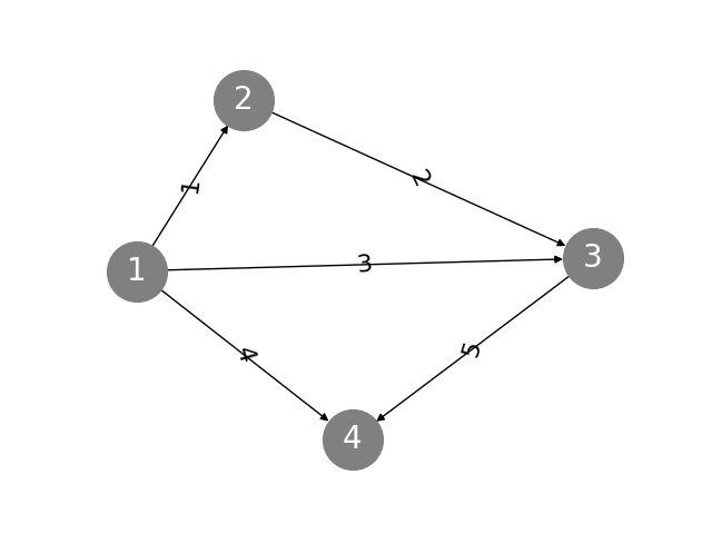
We can use an incidence matrix to describe that graph.
$$
\begin{bmatrix}
-1 & 1 & 0 & 0 \\
0 & -1 & 1 & 0 \\
-1 & 0 & 1 & 0 \\
-1 & 0 & 0 & 1 \\
0 & 0 & -1 & 1
\end{bmatrix}
$$
Row m represents the edge m. And the column n represents the node n. -1 represents from where and 1 represent to where.
Are those columns in that matrix independent or dependent? What’s in the nullspace?
We can put it in $Ax=0$ to solve it.
$$
Ax =
\begin{bmatrix}
x_2 - x_1 \\
x_3 - x_2 \\
x_3 - x_1 \\
x_4 - x_1 \\
x_4 - x_3
\end{bmatrix}
=
\begin{bmatrix} 0 \\ 0 \\ 0 \\ 0 \\ 0 \end{bmatrix}
$$
We can get $x=c\begin{bmatrix} 1 \\ 1 \\ 1 \\ 1 \\ 1 \end{bmatrix}$. And $dim(N(A))=1$.
So what can it be used in application?
Assume that the graph is a circuit, and each node has potential $x$. Then $Ax$ gives potential differences across the edges.
Note that potential difference make circuit flows. So the nullspace tells that what $x$ make circuit not flow.
The rank of $A$ is $rank(A)=n-r=4-1=3$. So there are three independent columns in that matrix.
Then get the left nullspace. $dim(N(A^T))=m-r=5-3=2$.
$$
A^T y =
\begin{bmatrix}
-1 & 0 & -1 & -1 & 0 \\
1 & -1 & 0 & 0 & 0 \\
0 & 1 & 1 & 0 & -1 \\
0 & 0 & 0 & 1 & 1
\end{bmatrix}
\begin{bmatrix} y_1 \\ y_2 \\ y_3 \\ y_4 \\ y_5 \end{bmatrix}
=
\begin{bmatrix} 0 \\ 0 \\ 0 \\ 0 \end{bmatrix}
$$
We can consider $y_i$ as current on the edge. Ohm’s Law says the current equals some number(conductance or $\frac{1}{resistance}$) times the potential drop.
Each row of $A^T$ tells that the current from each edge flows in or flows out. For example, row 1 tells considering node 1, current flows out through edge 1, 3 and 4.
$A^T y = 0$ tells that the current flowing into a node must be equal to the current flowing out of it. It is known as Kirchhoff’s Current Law(KCL).
To get the basis for $N(A^T)$, we can deal with matrix by elimination, or simply by thinking.
If you know Kirchhoff’s Voltage Law(KVL), you can draw 3 loops(two small loops and a big loop) in the graph. Assume that every resistance on each edge is 1 and the current is 1, then if the direction of the loop we drew is different from the direction of current, we let that y be -1, otherwise 1. Let other current be zero.
The equations form of $A^T y = 0$ is
$$
\begin{cases}
-y_1 &+ y_3 &- y_4 &= 0 \\
& \quad y_1 &- y_2 &= 0 \\
\quad y_2 &+ y_3 &- y_5 &= 0 \\
& \quad y_4 &+ y_5 &= 0
\end{cases}
$$
The graph can be redrawn as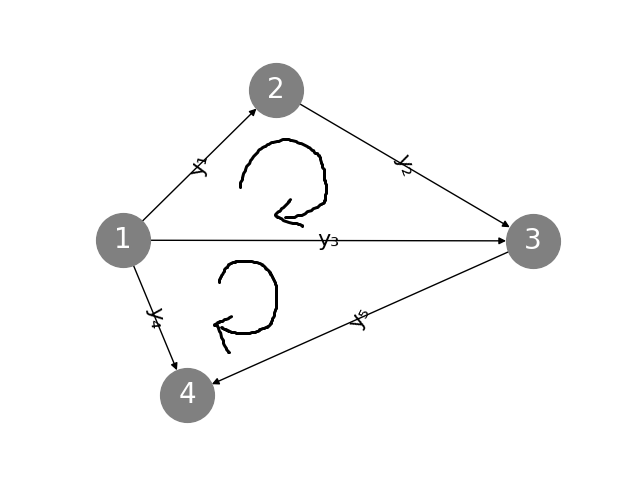
Start with loop $y_1 \rightarrow y_2 \rightarrow y_3 \rightarrow y_1$, let $y_1=1$, then $y_2=1,\ y_3=-1$. Let others($y_4$ and $y_5$) be zero. And we got one of the basis for $N(A^T)$: $\begin{bmatrix} 1 \\ 1 \\ -1 \\ 0 \\ 0 \end{bmatrix}$
Then the loop $y_1 \rightarrow y_3 \rightarrow y_4 \rightarrow y_1$. Let $y_3=1$, then $y_4-=1,\ y_5=1$. Let others be zero. And we got $\begin{bmatrix} 0 \\ 0 \\ 1 \\ -1 \\ 1 \end{bmatrix}$
What about the big loop? We can get $\begin{bmatrix} 1 \\ 1 \\ 0 \\ -1 \\ 1 \end{bmatrix}$, but it’s not a basis because it’s not independent. It’s a linear combination of two basis we have got above. In other words, the current on the big loop can be figured out by two small loops. We can add two small loop together and then $y_3$ is counterbalanced.
So in conclusion, the basis of $N(A^T)$ are $\begin{bmatrix} 1 \\ 1 \\ -1 \\ 0 \\ 0 \end{bmatrix}$ and $\begin{bmatrix} 0 \\ 0 \\ 1 \\ -1 \\ 1 \end{bmatrix}$.
The pivot columns of $A^T$ are $\begin{bmatrix} -1 \\ 1 \\ 0 \\ 0 \end{bmatrix}$, $\begin{bmatrix} 0 \\ -1 \\ 1 \\ 0 \end{bmatrix}$ and $\begin{bmatrix} -1 \\ 0 \\ 0 \\ 1 \end{bmatrix}$. They are edge 1, 2 and 4.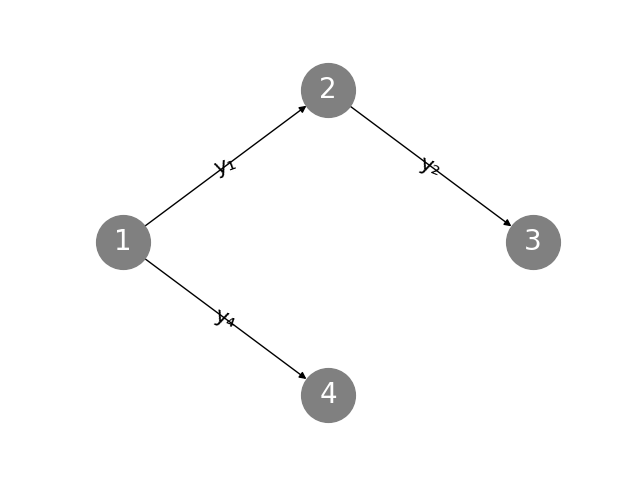
In this graph, there is no loop. We call it tree.
In this example, $dim(N(A^T)) = m-r$ equals the amount of loops, $m$ equals the amount of edges, and $r$ equals $(\text{the amount of nodes }-1)$. Notice that we don’t consider “the big loop” mentioned above as a loop.
Actually, for any graphs, $\text{nodes} - \text{edges} - \text{loops} = 1$. This is called Euler’s formula.
The trace of $A^T A$ equals to amount of edges connecting to each node.
In the example above, for node 1 there are 3 edges; for node 2 there are 2 edges; for node 3 there are 3 edges; for node 4 there are 2 edges. So $tr(A^T A)=3+2+3+2=10$
Notice that $A^T A$ is a symmetric matrix.
12. Orthogonal Vectors and Matrices
12.1 Orthogonal Vectors
The word orthogonal is another word of perpendicular. It means in n-dimensional space, the angle between those vectors is 90 degrees.
If there are two vectors $\vec v$, $\vec w$ and if $\vec v \cdot \vec w = 0$, we say they are orthogonal vectors.
If we draw the triangle consist of two orthogonal vectors $\vec v$, $\vec w$ and the hypotenuse $\vec v + \vec w$. We have Pythagorean theorem:
$$
|\vec v|^2 + |\vec w|^2 = |\vec v + \vec w|^2
$$
We can write the dot product as matrix multiplication: $x^T y = 0$
Then we can write the Pythagorean theorem as
$$
\begin{align}
x^T x + y^T y &= (x+y)^T(x+y) \\
&= x^T x + y^T y + x^T y + y^T x
\end{align}
$$
So we can get
$$
\begin{align}
x^T y + y^T x = 0
\end{align}
$$
For vectors, $x^T y = y^T x = 0$. So we can get
$$
2 x^T y = 0
$$
So we have checked that the relation between Pythagorean theorem and orthogonal vectors.
Then the subspace.
Is there a subspace orthogonal to other subspace?
If subspace $S$ orthogonal to subspace $T$, then every vector in subspace $S$ is orthogonal to every vector in subspace $T$. So if $S$ and $T$ are 2-dimensional subspaces, then two plane spanned by two subspaces are perpendicular.
Prove that row space is orthogonal to nullspace.
We know if $x$ in nullspace, then $Ax=0$. And $Ax=0$ already tells us the row space is perpendicular to nullspace, because
$$
Ax=
\begin{bmatrix} row_1 \\ row_2 \\ \vdots \\ row_m \end{bmatrix}
\begin{bmatrix} x_1 \\ x_2 \\ \vdots \\ x_m \end{bmatrix}
=
\begin{bmatrix}
row_1 x \\
row_2 x \\
\vdots \\
row_m x
\end{bmatrix}
=
\begin{bmatrix} 0 \\ 0 \\ \vdots \\ 0 \end{bmatrix}
$$
When we multiply every row in matrix by $x$, equivalent to taking product of two vectors, it equals zero.
We say null space and row space are orthogonal complements in $\mathbb{R}^n$.
Null space contains all vectors perpendicular to row space.
For example, if we know $\begin{bmatrix} 1 & 2 & 2 & 3 \end{bmatrix}$ and $\begin{bmatrix} 1 & 3 & 3 & 2 \end{bmatrix}$ in space $S$, and we want to find a basis for $S^{\bot}$.
If $x$ is in $S^{\bot}$, then we have $\begin{bmatrix} 1 & 2 & 2 & 3 \end{bmatrix}x = 0$ and $\begin{bmatrix} 1 & 3 & 3 & 2 \end{bmatrix}x=0$.
Write in matrix form: $\begin{bmatrix} 1 & 2 & 2 & 3 \\ 1 & 3 & 3 & 2 \end{bmatrix}x = 0$.
Just eliminate the matrix: $\begin{bmatrix} 1 & 2 & 2 & 3 \\ 0 & 1 & 1 & -1 \end{bmatrix}x = 0$
And then get the nullspace: $\begin{bmatrix} 0 & -1 & 1 & 0 \end{bmatrix},\begin{bmatrix} -5 & 1 & 0 & 1 \end{bmatrix}$. These two vectors are the basis we need to find.
Think of this: can every $\vec v$ in $\mathbb{R}^4$ be written uniquely in terms of $S$ and $S^{\bot}$?
If so, there must be unique $c_1,\ c_2,\ c_3,\ c_4$ to let
$$
\vec v=
c_1\begin{bmatrix} 1 \\ 2 \\ 2 \\ 3 \end{bmatrix} +
c_2\begin{bmatrix} 1 \\ 3 \\ 3 \\ 2 \end{bmatrix} +
c_3\begin{bmatrix} 0 \\ -1 \\ 1 \\ 0 \end{bmatrix} +
c_4\begin{bmatrix} -5 \\ 1 \\ 0 \\ 1 \end{bmatrix}
$$
We can write it into a matrix form:
$$
\begin{bmatrix}
1 & 1 & 0 & -5 \\
2 & 3 & -1 & 1 \\
2 & 3 & 1 & 0 \\
3 & 2 & 0 & 1
\end{bmatrix}
\begin{bmatrix} c_1 \\ c_2 \\ c_3 \\ c_4 \end{bmatrix}
=
\vec v
$$
If we can find it, these four vectors are linear independent, meaning the matrix must be invertible. And it is.
12.2 Projection onto Subspaces and Projection Matrices
Imagine that there are two vectors $\vec a$ and $\vec b$. How to get the vector $\vec p$ which is the projection of $\vec b$ onto $\vec a$?
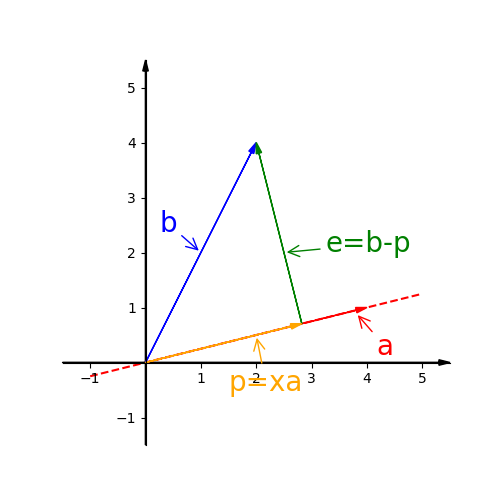
See this picture, we can get $a^T(b-p)=a^T(b-xa)=0$ because the dot product of two perpendicular vectors is zero.
Simply this equation, then we can get $a^T b = x a^T a$.
Notice that $x$ is a number. And the dot products $a^T b$ and $a^T a$ are also numbers.
So $\begin{equation} x = \cfrac{a^T b}{a^T a} \end{equation}$.
The projection vector is $\begin{equation} p = ax = a\cfrac{a^T b}{a^T a} \end{equation}$. (Intentionally put the number $x$ on the right)
Suppose we scale the vector $\vec b$ by some number $k$, then we can know from the equation that the projection will also be scaled by number $k$.
Suppose we scale the vector $\vec a$, the projection will not be changed at all.
If we want to find a matrix to describe the projection like $p = Pb$, what is the matrix?
From the equation we can find that
$$
P=\cfrac{a a^T}{a^T a}=\underbrace{\cfrac{1}{a^T a}}_{\text{number}} \underset{\underbrace{\underset{\quad\quad}{\quad\quad}}_{\scriptsize\textstyle\text{matrix}}}{a a^T}
$$
If $a$ is a n-dimensional vector, then $P$ is a nxn matrix.
Obviously $P$ is a symmetric matrix because $A^T A$ is symmetric for any matrix $A$.
If we square the matrix $P$, meaning take the projection twice $p=PPb$, then the projection is still $p$. So $P^2=P$.
So why projection? What can it be used in solving problem?
Think about the system of equations $Ax=b$. It may have no solution, i.e. there may be no linear combination of vectors in columns of $A$ to produce the vector $b$, i.e. again $Ax$ is always in the column space of $A$ but $b$ may not be in the column space of $A$.
So we can just get the closest solution. It may sound wierd. There is no solution, why getting the closest solution?
For example in 3-dimensional space, there is a plane spanned by the column vectors in $A$. And the vector $b$ point at somewhere but not in to the plane. If we get the vector $e=b-p$ perpendicular to the plane, then the vector $p$ is in the plane.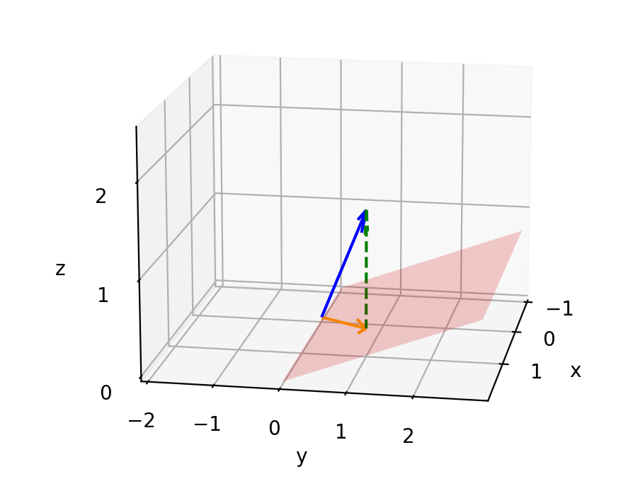
So we get a vector $p$, the projection of $b$ onto the column space, and then solve $A\hat x=p$ instead.
The key to find $\hat x$ for $p=A\hat x$ is that $b-A\hat x$ is perpendicular to the plane.
So we have $a_i^T(b-A\hat x)=0$. $a_i$ is a column vector in the column i of $A$.
Write in matrix form:
$$
A^T(b-A\hat x) =
\begin{bmatrix} a_1^T \\ a_2^T \\ \vdots \\ a_n^T \end{bmatrix}
(b-A\hat x)=
\begin{bmatrix} 0 \\ 0 \\ \vdots \\ 0 \end{bmatrix}
$$
We know if $Ax=0$ then $x$ is in the nullspace. So If $A^Tx=0$ then $x$ is in $N(A^T)$.
Therefore $e=(b-A\hat x)$ is in $N(A^T)$ and is perpendicular to $C(A)$.
Simplify the equation, then $A^T A\hat x = A^T b$, then $\hat x = (A^T A)^{-1} A^T b$.
So $p=A\hat x= A(A^T A)^{-1} A^T b$. The part $A(A^T A)^{-1} A^T$ is equivalent to $\begin{gather} \cfrac{a a^T}{a^T a} \end{gather}$. So the projection matrix $P=A(A^T A)^{-1} A^T$.
Notice that we cannot unfold $(A^T A)^{-1}$ to $A^{-1}(A^T)^{-1}$ and then get $A A^{-1}(A^T)^{-1} A^T=I$ because the matrix $A$ may not be a square matrix.
If $b$ is in column space, them $Pb=b$.
If $b$ is perpendicular to the column space, them $Pb=0$.
12.3 Least Squares
A classical usage of projection is the least squares fitting by a line.
For example, there are three point (1, 1), (2, 2), (3, 2).
We cannot find a line($b=C+Dt$) through those three point, because we cannot find a solution for
$$
\begin{cases}
C + D = 1 \\
C + 2D = 2 \\
C + 3D = 2
\end{cases}
$$
Write in matrix form:
$$
\begin{bmatrix}
1 & 1 \\
1 & 2 \\
1 & 3
\end{bmatrix}
\begin{bmatrix} C \\ D \end{bmatrix}
=
\begin{bmatrix} 1 \\ 2 \\ 2 \end{bmatrix}
$$
It has no solution, but we can find the best or closest solution for it.
$Ax=b$ cannot be solved, but magically $A^T A\hat x = A^T b$ is solvable.
The error(difference) between $b$ and the best solution is $e$, where $|e|^2 = |Ax-b|^2$. What we need to do is to minimise $e_1^2+e_2^2+e_3^3$. This operation is called linear regression.
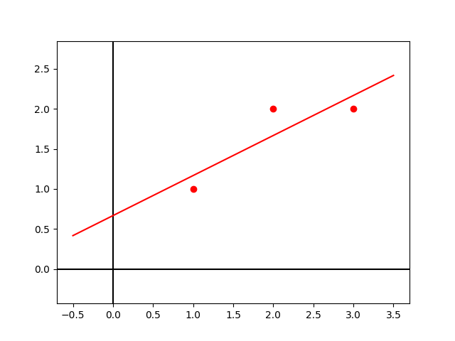
If there is one (or more) of these points is obviously far way off comparing with other points, we remove it to get the best line.
To find $\hat x$ and $p$, we just solve the equation $A^T A\hat x = A^T b$.
Remember that $b=e+p$, $p=Pb$, $e$ is in $N(A^T)$.
Then we get $\hat x = \begin{bmatrix} \cfrac{2}{3} \\ \cfrac{1}{2} \end{bmatrix}$, meaning the best line is $\begin{equation} y=\cfrac{2}{3} + \cfrac{1}{2}t \end{equation}$
So we can get $e=Ax-b=\begin{bmatrix} -\cfrac{1}{6} \\ \cfrac{1}{3} \\ -\cfrac{1}{6} \end{bmatrix}$ and $p=b-e=\begin{bmatrix} \cfrac{7}{6} \\ \cfrac{5}{3} \\ \cfrac{13}{6} \end{bmatrix}$
The error $e$ is perpendicular to $p$ and $C(A)$. $e \cdot p = 0$
12.4 Orthogonal Matrices
If we have orthogonal basis(also called orthonormal vectors) $q_1,\ q_2,\ \cdots,\ q_n$, then
$$
q_i^T q_j =
\begin{cases}
0 \quad \text{if } i \ne j \\
1 \quad \text{if } i = j
\end{cases}
$$
For orthonormal vectors, they are unit vectors, i.e. the length of each vector is 1.
If we have orthogonal matrix $Q=\begin{bmatrix} \big| & & \big| \\ q_1 & \cdots & q_n \\ \big| & & \big| \end{bmatrix}$, then $Q^T Q = \begin{bmatrix} 1 \\ & 1 \\ & & \ddots \\ & & & 1 \end{bmatrix} = I$.
The matrix $Q$ is also called orthonormal matrix.
If $Q$ is square, then $Q^T Q=I$ tells us $Q^T=Q^{-1}$.
Examples of orthogonal matrix:
- $\begin{bmatrix} 0 & 1 & 0 \\ 1 & 0 & 0 \\ 0 & 0 & 1 \end{bmatrix}$,
- $\begin{bmatrix} \cos\theta & -\sin\theta \\ \sin\theta & \cos\theta \end{bmatrix}$,
- $\begin{gather}\cfrac{1}{\sqrt{2}}\end{gather}\begin{bmatrix} 1 & 1 \\ 1 & -1 \end{bmatrix}$,
- $\begin{gather}\cfrac{1}{2}\end{gather}\begin{bmatrix} 1 & 1 & 1 & 1 \\ 1 & -1 & 1 & -1 \\ 1 & 1 & -1 & -1 \\ 1 & -1 & -1 & 1 \end{bmatrix}$,
- $\begin{gather}\cfrac{1}{3}\end{gather}\begin{bmatrix} 1 & -2 & 2 \\ 2 & -1 & -2 \\ 2 & 2 & 1 \end{bmatrix}$,
The length of each column vector is 1, and the column vectors are orthogonal.
Suppose $Q$ has orthonormal columns, how to find the projection matrix $P$ onto its column space? Remember that we have $Q^T Q=I$.
$$
P = Q(Q^T Q)^{-1}Q^T = QQ^T
$$
If Q is square, then $P = QQ^T = I$.
For $A^T A \hat x = A^T b$, let $A$ be $Q$, then $\hat x = Q^T b$.
Each component of $\hat x$ is
$$
\hat x_i = q_i^T b
$$
This is an important equation in mathematics. If we have orthonormal basis, then the the projection onto $x_i$ is $q_i^T b$.
Another way to prove $\hat x_i = q_i^T b$:
Suppose $p = p_1 + p_2 + \cdots + p_n$ are orthonormal basis, where $p_i \cdot p_j = \begin{cases} 0 \quad i \ne j \\ 1 \quad i=j \end{cases}$.
The projection onto $x$: $v = x_1 q_1 + x_2 q_2 + \cdots + x_n q_n$.
Then $q_1^T v = x_1 q_1^T q_1 + x_2 q_1^T q_2 + \cdots + x_n q_1^T q_n = x_1$.
Similarly, we can get $x_2 = q_2^T v$, …, $x_i = q_i^T v$.
12.5 Gram-Schmidt Orthogonalization
If we have two vectors $a$ and $b$ which are not orthogonal, the method to get orthogonal version is to get the vector $e$:
We can get the new vectors $A$ and $B$, then the orthonormal vectors $\begin{equation} q_1=\cfrac{A}{|A|},\ q_2=\cfrac{B}{|B|} \end{equation}$.
Firstly, we can let $A=a$. Then what we need to do is to find $B$ perpendicular to $A$.
We know $e=b-p$, so $\begin{gather} B=b-\cfrac{A^T b}{A^T A}A \end{gather}$.
If there are three vectors $a$, $b$ and $c$, how to get $C$?
We have already got $A$ and $B$. Now we have to get $C$ perpendicular to $A$ and $B$. Then $\begin{equation} q_1=\cfrac{A}{|A|},\ q_2=\cfrac{B}{|B|},\ q_3=\cfrac{C}{|C|} \end{equation}$.
$$
\begin{equation}
C = b-\cfrac{A^T c}{A^T A}A - \cfrac{B^T c}{B^T B}B
\end{equation}
$$
We use $A=LU$ to describe elimination, and we can also use a similar form $A=QR$ to describe orthonormalization.
If $A=\begin{bmatrix} a_1 & a_2 \end{bmatrix}$, then after orthonormalization $\begin{bmatrix} a_1 & a_2 \end{bmatrix} = \begin{bmatrix} q_1 & q_2 \end{bmatrix}\begin{bmatrix} a_1^T q_1 & a_2^T q_1 \\ a_1^T q_2 & a_2^T q_2 \end{bmatrix}$.
Since the new vector (like $q_2$) is perpendicular to the earlier (like $a_1$), so the dot product (like $a_1^T q_2$) is zero. So the matrix $R$ is an upper triangular matrix.
Example Question:
Find $q_1,\ q_2,\ q_3$(orthonormal) from $a,\ b,\ c$(columns of $A$). Then write $A$ as $QR$.
$
A =
\begin{bmatrix}
1 & 2 & 4 \\
0 & 0 & 5 \\
0 & 3 & 6
\end{bmatrix}
$
Solution:
$$
\begin{align}
q_1 &= \cfrac{a}{1} = \begin{bmatrix} 1 \\ 0 \\ 0 \end{bmatrix} \\
q_2’ &= b - e = b - (b \cdot q_1)q_1 \\
&= \begin{bmatrix} 2 \\ 0 \\ 3 \end{bmatrix} - 2\begin{bmatrix} 1 \\ 0 \\ 0 \end{bmatrix} = \begin{bmatrix} 0 \\ 0 \\ 3 \end{bmatrix} \\
q_2 &= \cfrac{q_2’}{|q_2|} = \begin{bmatrix} 0 \\ 0 \\ 1 \end{bmatrix} \\
q_3’ &= c - (c \cdot q_1)q_1 - (c \cdot q_2)q_2 \\
&= \begin{bmatrix} 4 \\ 5 \\ 6 \end{bmatrix} - 4\begin{bmatrix} 1 \\ 0 \\ 0 \end{bmatrix} - 6\begin{bmatrix} 0 \\ 0 \\ 1 \end{bmatrix} = \begin{bmatrix} 0 \\ 5 \\ 0 \end{bmatrix} \\
q_3 &= \cfrac{q_3’}{|q_3|} = \begin{bmatrix} 0 \\ 1 \\ 0 \end{bmatrix}
\end{align}
$$
Then write as $A=QR$:
$$
\begin{bmatrix}
1 & 2 & 4 \\
0 & 0 & 5 \\
0 & 3 & 6
\end{bmatrix}
=
\begin{bmatrix}
1 & 0 & 0 \\
0 & 0 & 1 \\
0 & 1 & 0
\end{bmatrix}
\begin{bmatrix}
1 & 2 & 4 \\
0 & 3 & 6 \\
0 & 0 & 5
\end{bmatrix}
$$
12.6 Rotation Matrices and Reflection Matrices
A rotation matrix or a reflection matrices is always orthonormal matrices.
Because the length of every column vector in that matrix is 1. After transformation, all perpendicular basis are still perpendicular.
So the transformation won’t scale the space. It just rotates or reflects the space.
13. Properties of Determinants
13.1 Properties
We have learnt determinants before. There are several properties of determinants:
- $det(I) = 1$
- Exchanging two rows reverse the sign of determinant. For permutation matrix, the determinant is depended on the number of exchanging times: $det(P)=\begin{cases} 1 \quad & even \\ -1 \quad & odd \end{cases}$.
- $\begin{vmatrix} ta & tb \\ c &d \end{vmatrix} = t\begin{vmatrix} a & b \\ c & d \end{vmatrix}$
- $\begin{vmatrix} a+a’ & b+b’ \\ c & d \end{vmatrix} = \begin{vmatrix} a & b \\ c & d \end{vmatrix} + \begin{vmatrix} a’ & b’ \\ c & d \end{vmatrix}$
Notice that for the fourth property, it’s NOT true that $det(A+B) = det(A) + det(B)$.
- If there are two same rows in matrix $A$, then $det(A)=0$. Because if we exchange this two row, the matrix doesn’t change. So $PA=-A=A$, meaning that $A=0$.
- If we subtract $l \times row_i$ from $row_k$, the determinant doesn’t change.
$\begin{vmatrix} a & b \\ c-la & d-lb \end{vmatrix} = \begin{vmatrix} a & b \\ c & d \end{vmatrix} + \begin{vmatrix} a & b \\ -la & -lb \end{vmatrix} = \begin{vmatrix} a & b \\ c & d \end{vmatrix} - l\begin{vmatrix} a & b \\ a & b \end{vmatrix}=\begin{vmatrix} a & b \\ c & d \end{vmatrix}$ - If there are a row full of zeros in matrix $A$, then $det(A)=0$.
- If the matrix $A$ is an upper triangular matrix like $\begin{bmatrix} b_1 \\ 0 & b_2 \\ &&\ddots \\ 0 & 0 & \cdots & b_n \end{bmatrix}$, then $det(A)=b_1b_2 \cdots b_n$.
It tells us that we can eliminate the matrix to the upper triangular form, then multiply the pivots to get the determinant. - If the matrix $A$ is singular(not invertible), then $det(A)=0$. If that matrix is invertible(non-singular), then $det(A) =\ne 0$.
- $det(AB)=det(A)det(B)$.
So we have $\begin{gather} det(A^{-1}) = \cfrac{1}{det(A)} \end{gather}$. Because we know $A^{-1}A=I$, then $\begin{gather} det(I)=det(A^{-1}A)=det(A^-1)det(A) \end{gather}$. So $\begin{gather} det(A^-1)=\cfrac{det(I)}{det(A)}=\cfrac{1}{det(A)} \end{gather}$.
We can also get $det(A^2) = (det(A))^2$ and $det(2A) = 2^n det(A)$. - $det(A^T)=det(A)$. So the properties dealing with rows mentioned can be used for columns.
13.2 Cofactors
A 3x3 determinant can be calculated as
$$
\begin{align}
\begin{vmatrix} a_{11} & a_{12} & a_{13} \\ a_{21} & a_{22} & a_{23} \\ a_{31} & a_{32} & a_{33} \end{vmatrix}
&= a_{11}a_{22}a_{33}+a_{12}a_{23}a_{31}+a_{13}a_{21}a_{32}-a_{11}a_{23}a_{32}-a_{12}a_{21}a_{33}-a_{13}a_{22}a_{31} \\
&= a_{11}(a_{22}a_{33}-a_{23}a_{32})-a_{12}(a_{21}a_{33}-a_{23}a_{31})+a_{13}(a_{21}a_{32}-a_{22}a_{31}) \\
&=
a_{11} \begin{vmatrix} a_{22} & a_{23} \\ a_{32} & a_{33} \end{vmatrix} -
a_{12} \begin{vmatrix} a_{21} & a_{23} \\ a_{31} & a_{33} \end{vmatrix} +
a_{13} \begin{vmatrix} a_{21} & a_{22} \\ a_{31} & a_{32} \end{vmatrix} \\
&=
\begin{vmatrix} a_{11} & 0 & 0 \\ 0 & a_{22} & a_{23} \\ 0 & a_{32} & a_{33} \end{vmatrix} +
\begin{vmatrix} 0 & a_{12} & 0 \\ a_{21} & 0 & a_{23} \\ a_{31} & 0 & a_{33} \end{vmatrix} +
\begin{vmatrix} 0 & 0 & a_{13} \\ a_{21} & a_{22} & 0 \\ a_{31} & a_{32} & 0 \end{vmatrix}
\end{align}
$$
We define cofactor of $a_{ij}$ as $C_{ij}$, the determinant of (n-1)x(n-1) matrix with row i and column j erased, with the positive sign if $i+j$ is even or negative if $i+j$ is odd.
For example, cofactor of $a_{11}$ is $C_{11} = \begin{vmatrix} a_{22} & a_{23} \\ a_{32} & a_{33} \end{vmatrix}$. Cofactor of $a_{12}$ is $C_{12} = -\begin{vmatrix} a_{21} & a_{23} \\ a_{31} & a_{33} \end{vmatrix}$
Then we have cofactor formula along row 1: $det(A) = a_{11}C_{11} + a_{12}C_{12} + a_{13}C_{13}$.
The way we expand 3x3 matrix into the addition of entries times 2x2 matrices is called cofactor expansion or Laplace expansion.
We can also expand row 2, row 3, or even column i.
13.3 Use determinant to get $A^{-1}$
First, we define a cofactor matrix $C = \begin{bmatrix} C_{11} & C_{12} & \cdots & C_{1n} \\ C_{21} & C_{22} & \cdots & C_{2n} \\ \vdots & \vdots & \ddots & \vdots \\ C_{n1} & C_{n2} & \cdots & C_{nn} \end{bmatrix}$.
Then we have $\begin{equation} A^{-1} = \cfrac{1}{det(A)}C^T \end{equation}$.
How to prove it?
First, simply it to $AC^T = det(A)I$. Then we just need to prove that left equals right.
For $AC^T$, write it into matrix form:
$$
\begin{align}
\begin{bmatrix}
a_{11} & a_{12} & \cdots & a_{1n} \\
a_{21} & a_{22} & \cdots & a_{2n} \\
\vdots & \vdots & \ddots & \vdots \\
a_{n1} & a_{n2} & \cdots & a_{nn}
\end{bmatrix}
\begin{bmatrix}
C_{11} & C_{21} & \cdots & C_{n1} \\
C_{12} & C_{22} & \cdots & C_{n2} \\
\vdots & \vdots & \ddots & \vdots \\
C_{1n} & C_{2n} & \cdots & C_{nn}
\end{bmatrix}
&=
\begin{bmatrix}
\sum\limits_{k=1}^n{a_{1k}C_{1k}} & \sum\limits_{k=1}^n{a_{1k}C_{2k}} & \cdots & \sum\limits_{k=1}^n{a_{1k}C_{nk}} \\
\sum\limits_{k=1}^n{a_{2k}C_{1k}} & \sum\limits_{k=1}^n{a_{2k}C_{2k}} & \cdots & \sum\limits_{k=1}^n{a_{2k}C_{nk}} \\
\vdots & \vdots & \ddots & \vdots \\
\sum\limits_{k=1}^n{a_{nk}C_{1k}} & \sum\limits_{k=1}^n{a_{nk}C_{2k}} & \cdots & \sum\limits_{k=1}^n{a_{nk}C_{nk}}
\end{bmatrix} \\
&=
\begin{bmatrix}
det(A) & 0 & \cdots & 0 \\
0 & det(A) & \cdots & 0 \\
\vdots & \vdots & \ddots & \vdots \\
0 & 0 & \cdots & det(A)
\end{bmatrix} \\
&=
det(A)I
\end{align}
$$
For diagonal entry(i,i), $\sum\limits_{k=1}^n{a_{ik}C_{ik}}$ is a cofactor expansion of column i for the matrix $A$. So it equals $det(A)$.
For other entry, if entries of a row (or column) are multiplied with cofactors of any other row (or column), then their sum is zero. Multiplying a row by the co-factors of any other row will mean that the row itself is duplicated in the determinant being evaluated. It is like calculating a determinant with two equal rows.
By the way, if the cofactor matrix of a nxn matrix $A$ is $A^*$, where $n>1$, then the determinant of the cofactor matrix $|A^*|=|A|^{n-1}$.
$A^*=|A|A^{-1}$
14. Difference Equations, Differential Equations and exp(At)
In this chapter, we use diagonalization to solve the problem.
A prerequisite knowledge of this chapter is derivative.
14.1 Difference Equation $u_{k+1}=Au_k$
Given a first order difference equation start with given vector $\vec u_0$, and $u_{k+1}=Au_k$, then $u_1=Au_0,\ u_2=A^2 u_0,\ \cdots,\ u_k=A^k u_0$.
To solve it, we expand $u_0$ to the linear combination of eigenvectors for matrix $A$
$$
u_0=c_1 x_1 + c_2 x_2 + \cdots + c_n x_n
$$
Then
$$
Au_0=c_1 \lambda_1 x_1 + c_2 \lambda_2 x_2 + \cdots + c_n \lambda_n x_n
$$
Write in matrix form:
$$
Au_0 =
\begin{bmatrix} x_1 & x_2 & \cdots & x_n\end{bmatrix}
\begin{bmatrix}
\lambda_1 & 0 & \cdots & 0 \\
0 & \lambda_2 & \cdots & 0 \\
\vdots & \vdots & \ddots & \vdots \\
0 & 0 & \cdots & \lambda_n
\end{bmatrix}
\begin{bmatrix} c_1 \\ c_2 \\ \cdots \\ c_n\end{bmatrix} =
S \Lambda c
$$
Then $Au_0 = S\Lambda S^{-1}u_0 = S\Lambda S^{-1}Sc = S\Lambda c$.
So $u_k = A^k u_0 = S\Lambda^{k}c=c_1\lambda_1^{k}x_1+c_2\lambda_2^{k}x_2+\cdots+c_n\lambda_n^{k}x_n$
14.2 Fibonacci Sequence
For Fibonacci Sequence $0, 1, 1, 2, 3, 5, 8, 13, …, F_n$, or $F_{k+2}=F_{k+1}+F_k$.
It’s a second order difference equation.
Let
$$
u_{k} = \begin{bmatrix} F_{k+1} \\ F_{k} \end{bmatrix}
$$
Then
$$
\begin{align}
u_{k+1} &= \begin{bmatrix} F_{k+2} \\ F_{k+1} \end{bmatrix} = \begin{bmatrix} F_{k+1} + F_{k} \\ F_{k+1} \end{bmatrix} \\
&= \begin{bmatrix} 1 & 1 \\ 1 & 0 \end{bmatrix}\begin{bmatrix} F_{k+1} \\ F_{k} \end{bmatrix}
\end{align}
$$
Let $A=\begin{bmatrix} 1 & 1 \\ 1 & 0 \end{bmatrix}$, then we have $u_{k+1}=Au_k$.
The eigenvalues for $A$: $\lambda_1=\frac{1+\sqrt{5}}{2},\ \lambda_2=\frac{1-\sqrt{5}}{2}$. The matrix is diagonalizable.
Then $F_{k}=c_1\left(\frac{1+\sqrt{5}}{2}\right)^{k}+c_2\left(\frac{1-\sqrt{5}}{2}\right)^{k}$.
When $k$ is a large number, we can get the approximation $F_{k} \approx c_1\left(\frac{1+\sqrt{5}}{2}\right)^{k}$ because the larger $k$ is, the closer to zero $c_2\left(\frac{1-\sqrt{5}}{2}\right)^{k}$ will be.
The eigenvectors are $\begin{bmatrix} \frac{1+\sqrt{5}}{2} \\ 1 \end{bmatrix}$ and $\begin{bmatrix} \frac{1-\sqrt{5}}{2} \\ 1 \end{bmatrix}$.
The initial $u_0=\begin{bmatrix} F_1 \\ F_0 \end{bmatrix} = \begin{bmatrix} 1 \\ 0 \end{bmatrix}$. In this case we can calculate $c$ from $\begin{bmatrix} 1 \\ 0 \end{bmatrix} = c_1 x_1 + c_2 x_2$. The result is $c_1=\frac{\sqrt{5}}{5},\ c_2=-\frac{\sqrt{5}}{5}$
Then we can get from $A^k=S\Lambda^k S^{-1}$ that
$$
\begin{align}
u_k &= A^k u_0 = S \Lambda^k S^{-1} Sc \\
&= \begin{bmatrix} \frac{1+\sqrt{5}}{2} & \frac{1-\sqrt{5}}{2} \\ 1 & 1 \end{bmatrix}
\begin{bmatrix} \left(\frac{1+\sqrt{5}}{2}\right)^k & 0 \\ 0 & \left(\frac{1-\sqrt{5}}{2}\right)^k \end{bmatrix}
\begin{bmatrix} \frac{\sqrt{5}}{5} \\ -\frac{\sqrt{5}}{5} \end{bmatrix} \\
&= \begin{bmatrix} c_1\lambda_1^{k+1} + c_2 \lambda_2^{k+1} \\ c_1\lambda_1^k + c_2\lambda_2^k \end{bmatrix}
\end{align}
$$
From $u_{99} = \begin{bmatrix} F_{k+1} \\ F_{99} \end{bmatrix}$ we can know that $F_{k}=c_1\lambda_1^k+c_2\lambda_2^k$.
So $u_k = c_1\lambda^k x_1 + c_2\lambda^k x_2$.
14.3 Differential Equations $\frac{\mathrm{d}u}{\mathrm{d}t}=Au$
For example
$$
\begin{cases}
\frac{\mathrm{d}u_1}{\mathrm{d}t} &= -u_1+2u_2 \\
\frac{\mathrm{d}u_2}{\mathrm{d}t} &= u_1-2u_2
\end{cases}
$$
Given an initial condition $u(0) = \begin{bmatrix} 1 \\ 0 \end{bmatrix}$.
The coefficient matrix is $A = \begin{bmatrix} -1 & 2 \\ 1 & -2 \end{bmatrix}$.
Initial condition $t=0$: $u(0) = \begin{bmatrix} u_1 \\ u_2 \end{bmatrix} = \begin{bmatrix} 1 \\ 0 \end{bmatrix}$.
Firstly, we get the eigenvalues of the matrix $A$. They are $\lambda_1=0,\ lambda_2=-3$.
The eigenvectors are $x_1 = \begin{bmatrix} 2 \\ 1 \end{bmatrix}$ for $\lambda_1$ and $\ x_2 = \begin{bmatrix} 1 \\ -1 \end{bmatrix}$ for $\lambda_2$.
Then the general solution is $u(t) = c_1 e^{\lambda_1t}x_1 + c_2 e^{\lambda_2t}x_2$.
But why? Let’s check it.
It means $e^{\lambda_1 t}$ is a solution of $\frac{\mathrm{d}u}{\mathrm{d}t}=Au$. So we just plug in $e^{\lambda_1 t}x_1$ to the left side, which means to take the $t$ derivative.
Then the left side becomes $\lambda_1 e^{\lambda_1 t}x_1$. The right side becomes $Ae^{\lambda_1 t}x_1$. So we have
$$
\lambda_1 e^{\lambda_1 t}x_1 = Ae^{\lambda_1 t}x_1
$$
Simplify it, then we get $\lambda_1 x_1 = A x_1$, which is the equation we get eigenvalues. So the general solution has been checked.
We expand the general solution in matrix form:
$$
\begin{align}
u(t) &= c_1 e^{\lambda_1t}x_1 + c_2 e^{\lambda_2t}x_2 \\
&= c_1 e^{0t} x_1 + c_2 e^{-3t}x_2 \\
&= c_1\begin{bmatrix} 2 \\ 1 \end{bmatrix} + c_2 e^{-3t}\begin{bmatrix} 1 \\ -1 \end{bmatrix}
\end{align}
$$
Then get the $c_1$ and $c_2$ from initial condition.
When $t=0$,
$$
u(0) = \begin{bmatrix} 1 \\ 0 \end{bmatrix}
= c_1\begin{bmatrix} 2 \\ 1 \end{bmatrix} + c_2\begin{bmatrix} 1 \\ -1 \end{bmatrix}
$$
So $c_1=\frac{1}{3},\ c_2=\frac{1}{3}$.
Finally, the solution is $u(t) = \frac{1}{3}\begin{bmatrix} 2 \\ 1 \end{bmatrix} + \frac{1}{3}e^{-3t}\begin{bmatrix} 1 \\ -1 \end{bmatrix}$.
When time $t$ increases from 0, the steady state $u(\infty) = \begin{bmatrix} \frac{2}{3} \\ \frac{1}{3} \end{bmatrix}$.
14.4 Stability
In which case $u(t) \to 0$? In previous example we know it requires negative eigenvalues.
Suppose eigenvalues are complex numbers, then what’s the requirements of eigenvalues?
To let $u(t) \to 0$, we need $e^{\lambda t} \to 0$.
Let $\lambda = a + bi$, then we have $e^{(a + bi)t} = e^{at}e^{bit}$.
We know from Euler’s formula that $e^{ix} = \cos x + i\sin x$. So $e^{bit} = \cos(bx) + i\sin(bx)$.
The modulus of exponential of imaginary number is one:
$$
\begin{align}
|e^{ix}| &= |\cos x + i\sin x| \\
&= \sqrt{(\Re(\cos x + i\sin x))^2 + (\Im(\cos x + i\sin x))^2} \\
&= \sqrt{\cos^2 x + \sin^2 x} = 1
\end{align}
$$
So the imaginary part of the complex number is running around the unit circle. It just makes the number oscillating.
Therefore, we just need the real part of $\lambda$ be negative.
If we need a steady state, we need to let one of the eigenvalues be zero and others’ real part be negative.
If blowing up, one of the eigenvalues’ real part is positive.
In conclusion
- Stability: $\Re(\lambda) < 0$
- steady state: one $\lambda_k = 0$ and others $\Re(\lambda) < 0$
- Blowing up: any $\Re(\lambda) > 0$
A trick to judge the stability of 2x2 matrix $A$: $A$ is steady when $tr(A) < 0$ and $det(A) > 0$.
Proof:
For 2x2 matrix $A = \begin{bmatrix} a & b \\ c & d \end{bmatrix}$
$$
\begin{align}
tr(A) &= a + d = \lambda_1 + \lambda_2 \\
det(A) &= ad - bc = \lambda_1 \lambda_2 \\
\text{If }tr(A)<0 \text{ and }& det(A)>0 \text{, then } \begin{cases} \lambda_1 + \lambda_2 < 0 \\ \lambda_1 \lambda_2 < 0 \end{cases} \\
\text{Therefore } \begin{cases} \lambda_1 < 0 \\ \lambda_2 < 0 \end{cases} & \text{ , which fits the condition of stability}
\end{align}
$$
14.5 Exponential Matrix $e^{At}$
For differential equations $\frac{\mathrm{d}u}{\mathrm{d}t}=Au$, the general solution is
$$
u(t) = e^{At}u(0) = Se^{\Lambda t}S^{-1}u(0)
$$
What the meaning of $e^A$?
There is a Taylor series $e^x=\sum \frac{x^n}{n!}$.
It can also be used with $e^{At}$.
$$
e^{At}=I+At+\frac{(At)^2}{2}+\frac{(At)^3}{6}+\cdots+\frac{(At)^n}{n!}+\cdots
$$
So
$$
\begin{align}
e^{At} &= I + At + \frac{(At)^2}{2} + \frac{(At)^3}{6} + \cdots + \frac{(At)^n}{n!} + \cdots \\
&= SS^{-1} + S\Lambda S^{-1}t + \frac{S\Lambda^2S^{-1}}{2}t^2 + \frac{S\Lambda^3S^{-1}}{6}t^3 + \cdots + \frac{S\Lambda^nS^{-1}}{n!}t^n + \cdots \\
&= S\left(I + \Lambda t + \frac{\Lambda^2t^2}{2} + \frac{\Lambda^3t^3}{3} + \cdots + \frac{\Lambda^nt^n}{n} + \cdots\right)S^{-1} \\
&= Se^{\Lambda t}S^{-1}
\end{align}
$$
The Taylor expansion for $e^{At}$ is always true. But for $e^{At} = Se^{\Lambda t}S^{-1}$, the matrix $A$ must be diagonlizable.
We can write $e^{\Lambda t}$ as matrix form:
$$
e^{\Lambda t} =
\begin{bmatrix}
e^{\lambda_1 t} & 0 & \cdots & 0 \\
0 & e^{\lambda_2 t} & \cdots & 0 \\
\vdots & \vdots & \ddots & \vdots \\
0 & 0 & \cdots & e^{\lambda_n t}
\end{bmatrix}
$$
If $\Re(\lambda) < 0$, then it’s steady.
14.6 n Order Differential Equation
For second order differential equation $y’’ + by’ + ky = 0$, we can turn it into 2x2 first order just like what we have done with Fibonacci.
Let $u = \begin{bmatrix} y’ \\ y \end{bmatrix}$
Then
$
u’ = \begin{bmatrix} y’’ \\ y’ \end{bmatrix}
= \begin{bmatrix} -by’-ky \\ y’ \end{bmatrix}
= \begin{bmatrix} -b & -k \\ 1 & 0 \end{bmatrix}\begin{bmatrix} y’ \\ y \end{bmatrix}
$
For 5th order $y’’’’’+by’’’’+cy’’’+dy’’+ey’+f=0$
$$
\begin{bmatrix}
y’’’’’ \\ y’’’’ \\ y’’’ \\ y’’ \\ y’
\end{bmatrix}
=
\begin{bmatrix}
-b & -c & -d & -e & -f \\
1 & 0 & 0 & 0 & 0 \\
0 & 1 & 0 & 0 & 0 \\
0 & 0 & 1 & 0 & 0 \\
0 & 0 & 0 & 1 & 0
\end{bmatrix}
\begin{bmatrix}
y’’’’ \\ y’’’ \\ y’’ \\ y’ \\ y
\end{bmatrix}
$$
For n order, we can still do it like this.
Then get the eigenvalues and eigenvectors and solve the question like what we have done with first order and Fibonacci.
Take $y’’’ + 2y’’ - y’ - 2y = 0$ as example.
Let $u(t) = \begin{bmatrix} y’’ \\ y’ \\ y \end{bmatrix}$
Then
$$
u’(t) = \begin{bmatrix} y’’’ \\ y’’ \\ y’ \end{bmatrix}
= \begin{bmatrix} -2 & 1 & 2 \\ 1 & 0 & \\ 0 & 1 & 0 \end{bmatrix}\begin{bmatrix} y’’ \\ y’ \\ y \end{bmatrix}
= Au(t)
$$
Then get the eigenvalues and eigenvectors.
$$
\begin{align}
det(A-\lambda I) &= \begin{vmatrix} -2-\lambda & 1 & 2 \\ 1 & -\lambda & \\ 0 & 1 & -\lambda \end{vmatrix} \\
&= (1-\lambda)(1+\lambda)(2+\lambda) \\
\text{for }\lambda_1=1 & \quad x_1 = \begin{bmatrix} 1 & 1 & 1 \end{bmatrix}^T \\
\text{for }\lambda_2=-1 & \quad x_2 = \begin{bmatrix} 1 & -1 & 1 \end{bmatrix}^T \\
\text{for }\lambda_3=-2 & \quad x_3 = \begin{bmatrix} 4 & -2 & 1 \end{bmatrix}^T
\end{align}
$$
Now we have got everything we need in order to create the general solution for $u(t)$.
$$
\begin{align}
u(t) &= c_1 e^t x_1 + c_2 e^{-t} x_2 + c_3 e^{-2t} x_3 \\
y(t) &= c_1 e^t + c_2 e^{-t} + c_3 e^{-2t}
\end{align}
$$
The choices of $c_1,\ c_2,\ c_3$ are arbitrary.
What about $exp(At)$?
For matrix $A$,
$$
\begin{gather}
S = \begin{bmatrix} x_1 & x_2 & x_3 \end{bmatrix} = \begin{bmatrix} 1 & 1 & 4 \\ 1 & -1 & -2 \\ 1 & 1 & 1 \end{bmatrix} \\
e^{\Lambda t} =
\begin{bmatrix}
e^t & & \\
& e^{-t} & \\
& & e^{-2t}
\end{bmatrix}
\end{gather}
$$
Therefore
$$
\begin{align}
exp(At) &= S e^{\Lambda t} S^{-1} \\
&=
\begin{bmatrix}
\frac{1}{6}e^t - \frac{1}{2}e^{-t} + \frac{4}{3}e^{-2t} \quad & \frac{1}{2}e^t - \frac{1}{2}e^{-t} \quad & \frac{1}{3}e^t + e^{-t} - \frac{4}{3}e^{-2t} \\
\frac{1}{6}e^t + \frac{1}{2}e^{-t} - \frac{2}{3}e^{-2t} \quad & \frac{1}{2}e^t + \frac{1}{2}e^{-t} \quad & \frac{1}{3}e^t - e^{-t} + \frac{2}{3}e^{-2t} \\
\frac{1}{6}e^t - \frac{1}{2}e^{-t} + \frac{1}{3}e^{-2t} \quad & \frac{1}{2}e^t - \frac{1}{2}e^{-t} \quad & \frac{1}{3}e^t + e^{-t} - \frac{1}{3}e^{-2t}
\end{bmatrix}
\end{align}
$$
15. Markov Matrices and Fourier Series
15.1 Markov Matrices
15.1.1 What is Markov Matrix
A Markov matrix is a matrix with all entries $\geqslant 0$ and the sum of every entry on its column is 1.
Markov matrix is used in probability.
The properties of Markov matrix:
- $\lambda=1$ is an eigenvalue.
- The absolute value of all other eigenvalues are smaller than 1: $|\lambda_i| < 1$
The kth power of $A$:
$$
u_k = A^k u_0 = S\Lambda^k S^{-1}u_0 = S\Lambda^k S^{-1}Sc = S\Lambda^k c = c_1\lambda_1^k x_1 + c_2\lambda_2^k x_2 + \cdots + c_n\lambda_n^k x_n
$$
When one of the eigenvalue $\lambda_k = 1$ and others are zero, then when $k \to \infty$, the steady state is $u_k = c_1 x_1$.
For $A-I$, the sum of every entry on its column is 0, and $A-I$ is singular because $\begin{bmatrix} 1 \\ 1 \\ \vdots \\ 1 \end{bmatrix}$ is in $N(A^T)$, then the eigenvectors are in $N(A)$.
The eigenvalues of $A$ and $A^T$ are the same because for $A$ we have $det(A-\lambda I)=0$ and for $A^T$ we have $det((A-\lambda I)^T)=det(A^T-\lambda I^T)=det(A^T-\lambda I)=0$ which is the calculation for eigenvalues of $A^T$.
15.1.2 An Example for Application
Suppose that each year there are $10%$ of people move from California(Cal) to Massachusetts(Mas) and %20%% from Mas to Cal.
What will be after 100 years or more?
We can write a matrix to describe it: $A=\begin{bmatrix} 0.9 & 0.2 \\ 0.1 & 0.8 \end{bmatrix}$.
Suppose the initial population $u_0 = \begin{bmatrix} u_{cal} \\ u_{mass} \end{bmatrix}_0 = \begin{bmatrix} 0 \\ 1000 \end{bmatrix}$.
So we have $u_k = A^k u_0$.
Let $u(t)=c_1 \lambda_1^t x_1 + c_2 \lambda_2^t x_2$.
We know $\lambda_1=1$ is a eigenvalue of $A$, so another one $lambda_2=tr(A)-\lambda_1=0.7$.
For $\lambda_1=1$, the eigenvector is $x_1 = \begin{bmatrix} 2 \\ 1 \end{bmatrix}$.
For $\lambda_2=0.7$, the eigenvector is $x_2 = \begin{bmatrix} -1 \\ 1 \end{bmatrix}$.
To get the steady state, we have $\lambda_1=1$ so $u(\infty) = c_1\begin{bmatrix} 2 \\ 1 \end{bmatrix}$.
Since the initial state $u_0 = \begin{bmatrix} 0 \\ 1000 \end{bmatrix} = c_1 \begin{bmatrix} 2 \\ 1 \end{bmatrix} + c_2 (0.7)^0 \begin{bmatrix} -1 \\ 1 \end{bmatrix}$
Then we have $c_1 = \frac{1000}{3}$ and $c_2 = \frac{2000}{3}$.
So for initial condition, the steady state would be $u(\infty) = \begin{bmatrix} \frac{2000}{3} \\ \frac{1000}{3} \end{bmatrix}$.
15.1.3 Another Example
A particle jumps between positions A and B with the following probabilities: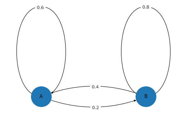
If it starts with A, what is the probability it is at A and B after
(i) 1 step
(ii) n steps
(iii) $\infty$ steps
Solution:
Let $M = \begin{bmatrix} 0.6 & 0.2 \\ 0.4 & 0.8 \end{bmatrix}$.
Initial position: $p_0 = \begin{bmatrix} 1 \\ 0 \end{bmatrix}$.
(i) 1 step: $p_1 = Mp_0 = \begin{bmatrix} 0.6 \\ 0.4 \end{bmatrix}$.
(ii) n steps: $p_n = M^n p_0$
We know $M=S \Lambda S^{-1}$.
Eigenvalues for $M$: $\lambda_1 = 1$ and $\lambda_2 = 0.4$.
Eigenvectors: for $\lambda_1$: $\begin{bmatrix} 1 \\ 2 \end{bmatrix}$; for $\lambda_2$: $\begin{bmatrix} 1 \\ -1 \end{bmatrix}$.
Then $\Lambda = \begin{bmatrix} 1 & 0 \\ 0 & 0.4 \end{bmatrix}$, $S = \begin{bmatrix} 1 & 1 \\ 2 & -1 \end{bmatrix}$, $S^{-1} = \frac{1}{3}\begin{bmatrix} 1 & 1 \\ 2 & -1 \end{bmatrix}$
So $p_n = M^n p_0 = S \Lambda^n S^{-1} p_0 = \frac{1}{3}\begin{bmatrix} 2(0.4)^n + 1 \\ -2(0.4)^n + 1 \end{bmatrix}$.
(iii) $\infty$ steps: $p_{\infty} = \frac{1}{3}\begin{bmatrix} 1 \\ 2 \end{bmatrix}$.
15.2 Fourier Series
The expansion of Fourier series:
$$
f(x) = a_0 + a_1\cos x + b_1\sin x + a_2\cos 2x + b_2\sin 2x + \cdots
$$
We can find the orthonormal elements sine and cosine, which is perpendicular and the length is 1. We just need to project it into an orthogonal basis.
Like $v^Tw=v_1w_1+v_2w_2+\cdots+v_nw_n=0$, we can take an inner product of functions. But functions are continuous, So the inner product is
$$
f^T g = \int f(x)g(x)\mathrm{d}x
$$
We can find that the function $f(x)$ has a period of $2\pi$, So
$$
f^T g = \int_0^{2\pi} f(x)g(x)\mathrm{d}x
$$
For $sin x cos x$:
$$
\int_0^{2\pi}\sin{x}\cos{x}\mathrm{d}x = \left.\frac{1}{2}\sin^2x\right|_0^{2\pi}=0
$$
For $f(x) cos x$:
$$
\int_0^{2\pi}f(x)\cos x\mathrm{d}x = a_1\int_0^{2\pi}\cos^2x\mathrm{d}x = a_1\pi
$$
So
$$
a_1 = \frac{1}{\pi}\int_0^{2\pi}f(x)\cos x\mathrm{d}x
$$
16. Complex Vectors, Complex Matrices and Fast Fourier Transform
16.1 Complex Vectors
A complex vector $z=\begin{bmatrix} z_1 \\ z_2 \\ \vdots \\ z_n \end{bmatrix}$, whose entries are complex number, is in $\mathbb{C}^n$.
To calculate the modulus of the real vector, we can use $|v|=\sqrt{v^T v}$.
But for complex vector, we cannot use this way because $z=\begin{bmatrix} 1 & i \end{bmatrix}$ for example $z^T z = 0$. However it can’t be zero.
To calculate the modulus of the complex vector, we should use the transpose of the conjugate one times the vector: $|z|=\sqrt{\bar{z}^T z}$
There is a symbol to describe transpose of conjugate: $z^H=\bar{z}^T$
$H$ pronounces Hermitian.
Then the modulus of complex vector $|z| = \sqrt{z^H z} = \sqrt{|z_1|^2 + |z_2|^2 + \cdots + |z_n|^2}$
For the inner product of complex vectors, we have $\bar{y}^T x = y^H x$.
16.2 Complex Matrices
For perpendicular complex unit vectors $q_1, q_2, \cdots, q_n$
$$
q_i^H q_j =
\begin{cases}
0 \quad i \ne j \\
1 \quad i = j
\end{cases}
$$
Pack them into matrix to make a complex orthogonal matrix $Q = \begin{bmatrix} \big| & \big| & & \big| \\ q_1 & q_2 & \cdots & q_n \\ \big| & \big| & & \big| \end{bmatrix}$, then
$$
Q^H Q = I
$$
The complex orthogonal matrix is called unitary matrix.
For complex matrices, the symmetric condition is $\bar{A}^T=A$, i.e. $A^H=A$.
An example of complex symmetric matrix: $\begin{bmatrix} 2 & 3+i \\ 3-i & 5 \end{bmatrix}$
16.3 Fourier Matrices
nxn Fourier matrix
$$
F_n =
\begin{bmatrix}
1 & 1 & 1 & \cdots & 1 \\
1 & w & w^2 & \cdots & w^{n-1} \\
1 & w^2 & w^4 & \cdots & w^{2(n-1)} \\
\vdots & \vdots & \vdots & \ddots & \vdots \\
1 & w^{n-1} & w^{2(n-1)} & \cdots & w^{(n-1)^2}
\end{bmatrix}
$$
$w$ is a special number whose $w^n=1$.
Actually, $\begin{equation}w= e^{\scriptsize{\cfrac{i2\pi}{2}}} \end{equation}$.
It’s on the unit circle. So $w = \cos\frac{2\pi}{n} + i\sin\frac{2\pi}{n}$.
See this 4x4 Fourier matrix. We let $w=i$,
$$
F_4 =
\begin{bmatrix}
1 & 1 & 1 & 1 \\
1 & i & i^2 & i^3 \\
1 & i^2 & i^4 & i^6 \\
1 & i^3 & i^6 & i^9
\end{bmatrix}
=
\begin{bmatrix}
1 & 1 & 1 & 1 \\
1 & i & -1 & -i \\
1 & -1 & 1 & -1 \\
1 & -i & -1 & i
\end{bmatrix}
$$
If we normalize this matrix, which is to make $F_4 = \frac{1}{2}\begin{bmatrix} 1 & 1 & 1 & 1 \\ 1 & i & -1 & -i \\ 1 & -1 & 1 & -1 \\ 1 & -i & -1 & i \end{bmatrix}$, then $F_4$ is orthonormal.
Then we have $F_4^H F_4 = I$, which means $F_4$ is a unitary matrix.
Actually all Fourier matrices are unitary matrix.
16.4 Fast Fourier Transform (FFT)
For a nxn Fourier matrix whose n is even, it can be decomposed to $\frac{n}{2}x\frac{n}{2}$.
For example
$$
F_8 =
\begin{bmatrix}
1 & 1 & 1 & 1 & 1 & 1 & 1 & 1 \\
1 & w & -i & w^3 & -1 & -w & i & -w^3 \\
1 & w^2 & -1 & -w^2 & 1 & w^2 & -1 & -w^2 \\
1 & w^3 & i & w & -1 & -w^3 & -i & -w \\
1 & −1 & 1 & −1 & 1 & −1 & 1 & −1 \\
1 & -w & -i & -w^3 & -1 & w & i & w^3 \\
1 & -w^2 & -1 & w^2 & 1 & -w^2 & -1 & w^2 \\
1 & -w^3 & i & -w & -1 & w^3 & -i & w
\end{bmatrix}
$$
Then permute all columns of $F_N$ with even indices in order ahead of columns with odd indices.
$$
\begin{align}
F_8 P_8 &= F_8
\begin{bmatrix}
1 & 0 & 0 & 0 & 0 & 0 & 0 & 0 \\
0 & 0 & 0 & 0 & 1 & 0 & 0 & 0 \\
0 & 1 & 0 & 0 & 0 & 0 & 0 & 0 \\
0 & 0 & 0 & 0 & 0 & 1 & 0 & 0 \\
0 & 0 & 1 & 0 & 0 & 0 & 0 & 0 \\
0 & 0 & 0 & 0 & 0 & 0 & 1 & 0 \\
0 & 0 & 0 & 1 & 0 & 0 & 0 & 0 \\
0 & 0 & 0 & 0 & 0 & 0 & 0 & 1
\end{bmatrix} \\
&=
\begin{bmatrix}
\begin{array}{cccc : cccc}
1 & 1 & 1 & 1 & 1 & 1 & 1 & 1 \\
1 & -i & -1 & i & w & w^3 & -w & -w^3 \\
1 & -1 & 1 & -1 & w^2 & -w^2 & w^2 & -w^2 \\
1 & i & -1 & -i & w^3 & w & -w^3 & -w \\
\hdashline
1 & 1 & 1 & 1 & 1 & 1 & 1 & 1 \\
1 & -i & -1 & i & -w & -w^3 & w & w^3 \\
1 & -1 & 1 & -1 & -w^2 & w^2 & -w^2 & w^2 \\
1 & i & -1 & -i & -w^3 & -w & w^3 & w
\end{array}
\end{bmatrix} \\
&=
\begin{bmatrix}
F_4 & D_4 F_4 \\
F_4 & -D_4 F_4
\end{bmatrix}
\end{align}
$$
In the last matrix, $D_4$ is a diagonal matrix $\begin{bmatrix} 1 & 0 & 0 & 0 \\ 0 & w & 0 & 0 \\ 0 & 0 & w^2 & 0 \\ 0 & 0 & 0 & w^3 \end{bmatrix}$.
For $D_4 F_4$, it stands for
$$
\begin{bmatrix}
1 & 1 & 1 & 1 \\
w & w^3 & -w & -w^3 \\
w^2 & -w^2 & w^2 & -w^2 \\
w^3 & w & -w^3 & -w
\end{bmatrix}
=
\begin{bmatrix} 1 & 0 & 0 & 0 \\ 0 & w & 0 & 0 \\ 0 & 0 & w^2 & 0 \\ 0 & 0 & 0 & w^3 \end{bmatrix}
\begin{bmatrix} 1 & 1 & 1 & 1 \\ 1 & -i & -1 & i \\ 1 & -1 & 1 & -1 \\ 1 & i & -1 & -i \end{bmatrix}
= D_4 F_4
$$
The total process can be written as
$$
F_8 = \begin{bmatrix} I & D_4 \\ I & -D_4 \end{bmatrix}\begin{bmatrix} F_4 & 0 \\ 0 & F_4 \end{bmatrix}P
$$
For a larger n, we can use this way to reduce the complexity of computation.
for example $F_{64}$, we can break them down into two $F_{32}$:
$$
F_{64} = \begin{bmatrix} I & D_{32} \\ I & -D_{32} \end{bmatrix}\begin{bmatrix} F_{32} & 0 \\ 0 & F_{32} \end{bmatrix}P_{32}
$$
Then break $F_{32}$ down into two $F_{16}$:
$$
F_{64} =
\begin{bmatrix} I_{32} & D_{32} \\ I_{32} & -D_{32} \end{bmatrix}
\begin{bmatrix} I_{16} & D_{16} & & \\ I_{16} & -D_{16} & & \\ & & I_{16} & D_{16} \\ & & I_{16} & -D_{16} \end{bmatrix}
\begin{bmatrix} F_{16} & & & \\ & F_{16} & & \\ & & F_{16} & \\ & & & F_{16} \end{bmatrix}
\begin{bmatrix} P_{16} & \\ & P_{16} \end{bmatrix}P_{32}
$$
The complexity becomes $\frac{n}{2}\log_2{n}$.
17. Symmetric Matrices and Positive Definiteness
17.1 Eigenvalues and Eigenvectors of Symmetric Matrices
For symmetric matrices $A^T=A$, there are two facts:
- The eigenvalues are real number
- The eigenvectors are perpendicular
So if the eigenvalues are repeated, we can still choose the hidden eigenvector perpendicular to others.
For diagonlizable matrix $A$, it can be $A = S\Lambda S^{-1}$.
Since the eigenvectors are perpendicular, the pack of eigenvectors $Q$ is an orthogonal matrix.
If we normalize the eigenvectors and pack them into a matrix, then we get orthonormal matrix $Q$.
For orthonormal matrix, we have $Q^{-1} = Q^T$. (Proof here)
So the symmetric matrix can be $A = Q\Lambda Q^{-1} = Q\Lambda Q^T$, which means $Q\Lambda Q^T$ is a symmetric matrix.
Now prove that the eigenvalues are real number.
To get eigenvalues, we have
$$ Ax = \lambda x \tag{1} $$
The conjugate $\bar A\bar x=\bar\lambda \bar x$.
We are just talking about real matrix, so $A\bar x=\bar\lambda \bar x$.
Then transpose the equation:
$$ \bar{x}^TA=\bar{x}^T\bar\lambda \tag{2} $$
Multiply both side of (1) by $\bar{x}^T$:
$$
\bar{x}^T Ax = \bar{x}^T \lambda x \tag{3}
$$
Multiply both side of (2) by $x^T$:
$$
\bar{x}^T Ax = \bar{x}^T \bar\lambda x \tag{4}
$$
Comparing (3) with (4), they have the same left side. So
$$
\bar{x}^T \lambda x=\bar{x}^T \bar\lambda x
$$
The conclusion is $\lambda = \bar\lambda$. So the eigenvalue $\lambda$ is real.
For $\bar{x}^T x$, we have
$$
\bar{x}^T x = \begin{bmatrix} \bar x_1 & \bar x_2 & \cdots & \bar x_n \end{bmatrix}\begin{bmatrix} x_1 \\ x_2 \\ \vdots \\ x_n \end{bmatrix}
= \bar{x_1}x_1 + \bar{x_2}x_2 + \cdots + \bar{x_n}x_n
$$
If $x_1 = a+ib$, then $\bar{x_1}x_1 = (a+ib)(a-ib) = a^2+b^2$.
Therefore, $\bar{x}^T x > 0$. And $\bar{x}^Tx$ is the square of the length of $x$.
If $A$ is a complex matrix, then the properties 1 and 2 is true when $A = \bar{A}^T$.
Go back to $A = Q \Lambda Q^T$. Don’t forget $Q$ is an orthonormal matrix we just prove above.
Let $q_i$ be the column vectors of $Q$, then
$$
\begin{align}
A &= Q\Lambda Q^T =
\begin{bmatrix} \big| & \big| & & \big| \\ q_1 & q_2 & \cdots & q_n \\ \big| & \big| & & \big| \end{bmatrix}
\begin{bmatrix} \lambda_1 & & & \\ & \lambda_2 & & \\ & & \ddots & \\ & & & \lambda_n \end{bmatrix}
\begin{bmatrix} \overline{\quad} & q_1^T & \overline{\quad} \\ \overline{\quad} & q_1^T & \overline{\quad} \\ & \vdots & \\ \overline{\quad} & q_1^T & \overline{\quad} \end{bmatrix}
&= \lambda_1 q_1 q_1^T + \lambda_2 q_2 q_2^T + \cdots + \lambda_n q_n q_n^T
\end{align}
$$
Notice that $q_1 q_1^T$ is NOT dot product. $\frac{q q^T}{q^T q}=q q^T$ is a projection matrix.
So every symmetric matrix is a combination of perpendicular projection matrices.
We know the eigenvectors of symmetric matrix are perpendicular. So if we pack the eigenvectors into a matrix then normalize it, we get an orthonormal matrix, which refers to rotation.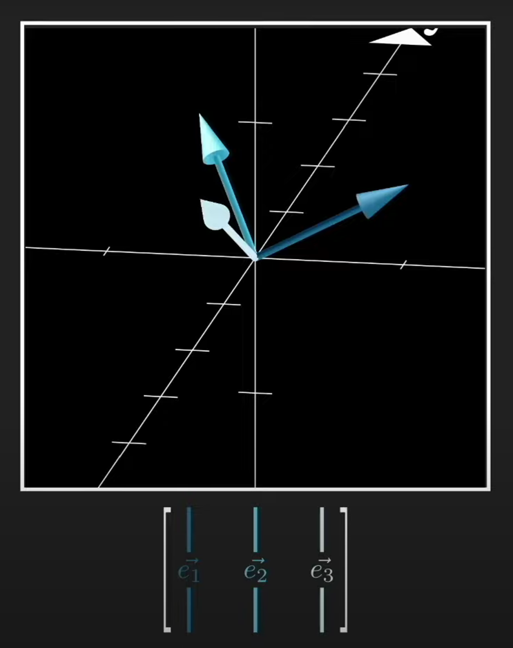
If we take the transpose of this rotation matrix, it rotates eigenvector to align with the standard basis.![]()
17.2 Positive Definiteness
Now talking about the sign of eigenvalues of symmetric matrices.
The sign of eigenvalues affects the stability of differential equation. So the sign is important.
But it’s easy to get that the sign of pivot is the same as the sign of eigenvalue.
If all eigenvalues are positive, we say that matrix is a positive definite matrix.
The positive definite matrix we are talking about is real matrix. It can be complex, but it’s out of this chapter.
To test whether the matrix is positive definite, we usually use the following four ways:
- All eigenvalues are larger than 0.
- The determinant of every leading principal submatrix is larger than 0.
For example, a 3x3 matrix $\begin{bmatrix} 1&2&3\\4&5&6\\7&8&9 \end{bmatrix}$ has three leading principal submatrix $\begin{bmatrix} 1 \end{bmatrix},\begin{bmatrix} 1&2\\4&5 \end{bmatrix},\begin{bmatrix} 1&2&3\\4&5&6\\7&8&9 \end{bmatrix}$ - Every pivot is larger than 0.
- $x^T Ax > 0$.
4 is the definition for real positive definite matrices. 1, 2, 3 can be used to verify it.
If $x^T Ax \geqslant 0$, the matrix $A$ is called positive semi-definite.
Take $A = \begin{bmatrix} 2 & 6 \\ 6 & a_4 \end{bmatrix}$ as an example.
If $a_4 = 18$, then $f(x_1, x_2) = x^T Ax = \begin{bmatrix} x_1 & x_2 \end{bmatrix}\begin{bmatrix} 2 & 6 \\ 6 & 18 \end{bmatrix}\begin{bmatrix} x_1 \\ x_2 \end{bmatrix} = 2x_1^2 + 12x_1 x_2 + 18x_2^2$.
What we get is called quadratic form, which has no linear part and constant part and is all 2 degree.
Let’s see what it looks like: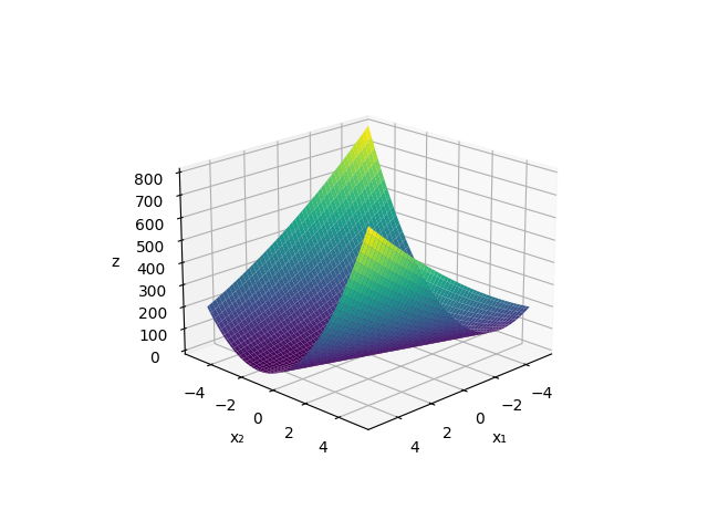
If $a_4 = 7$, then the matrix is absolutely NOT positive definite.
The graph of $x^T Ax = 2x_1^2 + 12x_1 x_2 + 18x_2^2$ looks like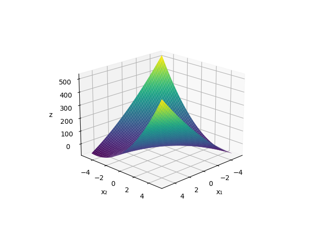
It goes through (0, 0, 0) and the purple part is lower than 0. It looks like a saddle.
If $a_4 = 20$, then the matrix is really a positive definite matrix.
The graph of $x^T Ax = 2x_1^2 + 12x_1 x_2 + 20x_2^2$ looks like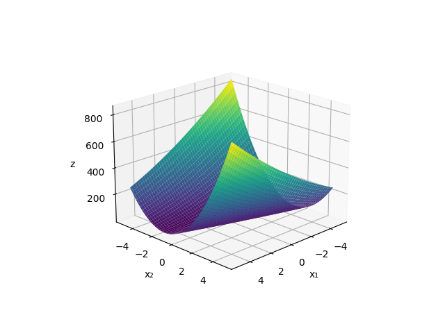
It’s positive everywhere except the point (0, 0, 0) which is the minimum. It looks like a paraboloid.
In calculus, the minimum is associated with $\frac{\mathrm{d}u}{\mathrm{d}x}=0, \frac{\mathrm{d}^2u}{\mathrm{d}x^2}>0$.
In linear algebra, we get minimum by ensuring that matrix of 2nd derivative is positive definite.
We can easily see whether it’s positive by making them into sum of squares.
For example, if $a_4=20$, then $2x_1^2+12x_1 x_2+20x_2^2 = 2(x_1+3x_2)^2+2x_2^2$ which is obviously larger than or equal 0.
If $a_4=7$, then $2x_1^2 + 12x_1 x_2 + 18x_2^2 = 2(x_1+3x_2)^2 - 11x_2^2$ which may be less than 0.
If $a_4=18$, then $2x_1^2 + 12x_1 x_2 + 18x_2^2 = 2(x_1+3x_2)^2$ is larger than or equal 0, but have more than one point equal zero.
Take a 3x3 matrix example $A = \begin{bmatrix} 2 & -1 & 0 \\ -1 & 2 & -1 \\ 0 & -1 & 2 \end{bmatrix}$.
The determinant of the leading principal submatrix are 2, 3 and 4.
The pivots are $2,\ \frac{3}{2},\ \frac{4}{3}$.
The eigenvalues are $\lambda_1=2-\sqrt 2,\ \lambda_2=2,\ \lambda_3=2+\sqrt 2$.
The quadratic form $f(x_1, x_2, x_3) = x^T Ax = 2x_1^2 + 2x_2^2 + 2x_3^2 - 2x_1 x_2 - 2x_2 x_3 > 0$.
The graph is a 4-dimensional paraboloid. If we cut through the picture at $f(x_1, x_2, x_3) = 1$, we will get a ellipsoid. And the directions of three axes are the same as three eigenvectors.
We can decompose $A$ to $A=Q\Lambda Q^T$, whose eigenvectors (in $Q$) tell the direction and the eigenvalues (in $\Lambda$) tell the length of axes. It’s called principal axis theorem.
17.3 Properties of Positive Definite
There are some facts of positive definite matrices:
- every positive definite matrix is invertible.
If $A$ is invertible, then $det(A)=\lambda_1\lambda_2\cdots\lambda_n \ne 0$.
And if $A$ is a positive definite matrix, we have $\lambda_i > 0$.
So $det(A)=\lambda_1\lambda_2\cdots\lambda_n > 0$, which proves the determinant of $A$ cannot be zero.
Hence $A$ is invertible. - The only positive definite projection matrix is $P=I$.
We know if $\lambda$ is an eigenvalue of $A$, then $\lambda^2$ is a eigenvalue of $A^2$. (Proof here)
For projection matrices, we have $P=P^2$. (Proof here)
Therefore from $Px = \lambda x$ we have $P^2 x = \lambda^2 x = Px = \lambda x$.
Because $x$ cannot be zero, then we have $\lambda^2 = \lambda$.
The solution is $\lambda_1=0$ and $\lambda_2=1$.
It means any projection matrices have only two eigenvalues 0 and 1.
If the projection matrix is positive definite, then the eigenvalues must be larger than 0. So the only eigenvalue of a positive definite projection matrix is 1.
The only symmetric matrix whose only eigenvalue is 1 can only be identity matrix.
Thus $P=I$.
The inverse of definite matrix is $A^{-1} = S\Lambda^{-1}S^{-1}$. Its eigenvalues are reciprocal of $A$’s. So the eigenvalues are positive, meaning that the inverse of a positive infinite matrix is still positive infinite.
For positive infinite matrix $A$ and $B$, to test whether $A + B$ is positive infinite, we let $x^T(A+B)x = x^T A x + x^T B x$.
Since $x^T A x > 0$, $x^T B x > 0$, then $x^T(A+B)x > 0$, meaning that $A + B$ is positive infinite.
For mxn nonsquare matrix $A$, we can get a symmetric matrix by $A^T A$, which is also a positive definite matrix.
Because $x^T(A^T A)x = x^T A^T A x = (Ax)^T (Ax)$ is a square of the length of vector $Ax$. To ensure that $|Ax|^2 > 0$, we just need to ensure that there is only zero vector in the nullspace of $A$, i.e. the column vectors in $A$ is linear independent ($rank(A)=n$). Then $A^T A$ is positive definite.
When eliminating with positive definite matrices, you don’t need to exchange two rows and the pivots will not be zero. So positive definite matrices are “good matrices” in computation.
18. Similar Matrices and Jordan Form
18.1 Similar Matrices
For nxn matrices $A$ and $B$, if $B=M^{-1}AM$ for some matrix $M$, then we say $A$ and $B$ is similar.
For example in diagonalization chapter we have $S^{-1}AS = \Lambda$, so $A$ is similar to $\Lambda$.
Similar matrices have the same eigenvalues.
Proof:
Suppose $Ax = \lambda x$ and $B = M^{-1}AM$
Then
$$
\begin{align}
Ax = A(M^{-1}M)x &= \lambda x \\
M^{-1}AMM^{-1}x &= \lambda M^{-1}x \\
BM^{-1}x &= \lambda M^{-1}x \\
B(M^{-1}x) &= \lambda (M^{-1}x)
\end{align}
$$
The matrix $B$ has the same $\lambda$ and the eigenvector is $M^{-1}x$.
18.2 Jordan Form
If two eigenvalues of $A$ are the same, it may not be possible to diagonalize because one eigenvector is “missing”.
Suppose $\lambda_1=\lambda_2=4$, we can write a lot of matrices like $\begin{bmatrix}4&0\\0&4\end{bmatrix}$ and $\begin{bmatrix}4&1\\0&4\end{bmatrix}$.
$\begin{bmatrix}4&0\\0&4\end{bmatrix}$ is similar to itself.
Other matrices like $\begin{bmatrix}4&1\\0&4\end{bmatrix}$, $\begin{bmatrix}4&0\\2&4\end{bmatrix}$, $\begin{bmatrix}5&1\\-1&3\end{bmatrix}$, they are similar.
But they are not diagonlizable. Because $\begin{bmatrix}4&0\\0&4\end{bmatrix}$ is similar to itself. They cannot be similar to the expected diagonlized matrix.
The matrix $\begin{bmatrix}4&1\\0&4\end{bmatrix}$, or generally the matrix
$$
J_i=
\begin{bmatrix}
\lambda_i & 1 & 0 & \cdots & 0 \\
0 & \lambda_i & 1 & \cdots & 0 \\
0 & 0 & \lambda_i & \ddots & \vdots \\
\vdots & \vdots & \vdots & \ddots & 1 \\
0 & 0 & 0 & \cdots & \lambda_i
\end{bmatrix}
$$
is called Jordan form.
A Jordan block $J_i$ has a repeated eigenvalue $\lambda_i$ on the diagonal, zeros below the diagonal and in the upper right-hand corner, and ones above the diagonal.
See this two matricecs:
$$\begin{bmatrix}0&1&0&0\\0&0&1&0\\0&0&0&0\\0&0&0&0\end{bmatrix},\ \begin{bmatrix}0&1&0&0\\0&0&0&0\\0&0&0&1\\0&0&0&0\end{bmatrix}$$
They have the same four eigenvectors (four zero), and have dimension 2 and rank 2. But surprisingly they are NOT similar.
We can break these matrices into their Jordan block:
$$
\begin{bmatrix}
\begin{array}{ccc|c}
0 & 1 & 0 & 0 \\
0 & 0 & 1 & 0 \\
0 & 0 & 0 & 0 \\ \hline
0 & 0 & 0 & 0
\end{array}
\end{bmatrix},\
\begin{bmatrix}
\begin{array}{cc|cc}
0 & 1 & 0 & 0 \\
0 & 0 & 0 & 0 \\ \hline
0 & 0 & 0 & 1 \\
0 & 0 & 0 & 0
\end{array}
\end{bmatrix}
$$
Two matrices may have the same eigenvalues and the same number of eigenvectors, but if their Jordan blocks are different sizes, those matrices can not be similar.
Jordan’s theorem says that every square matrix $A$ is similar to a Jordan matrix $J$, with Jordan blocks on the diagonal:
$$
\begin{bmatrix}
J_1 & 0 & \cdots & 0 \\
0 & J_2 & \cdots & 0 \\
\vdots & \vdots & \ddots & \vdots \\
0 & 0 & \cdots & J_d
\end{bmatrix}
$$
The number of blocks is the number of eigenvectors – there is one eigenvector per block.
If $A$ has $n$ distinct eigenvalues, it is diagonalizable and its Jordan matrix is the diagonal matrix $J = \Lambda$.
If $A$ has repeated eigenvalues and “missing” eigenvectors, then its Jordan matrix will have $n − d$ ones above the diagonal.
19. Singular Value Decomposition
19.1 What is it
Singular Value Decomposition (SVD) is a final and best factorization of a matrix:
$$
A = U\Sigma V^T
$$
where $U$ is orthogonal, $\Sigma$ is diagonal, and $B$ is orthogonal.
$A$ can be ANY matrix, regardless of the shape or the rank. it can unconditionally be decomposed.
When $A$ is positive definite, we can write $A=Q\Lambda Q^T$. It’s a special case of SVD, with $U=V=Q$.
For more general $A$, the SVD requires different matrices $U$ and $V$.
To understand SVD, firstly we need to recap the previous lectures in order to keep our brain from getting rusty.
Given any matrix $A$, then $A^T A$ is a symmetric matrix. (Proof here)
The eigenvectors of a symmetric matrix is perpendicular. (Proof here)
If we pack those eigenvectors into a matrix $S$, we get an orthogonal matrix which implies rotation. It rotates the basis to the eigenvectors.
The transpose of that matrix $S^T$ rotates the eigenvectors to align with the standard basis.
Then we let the matrix $U$ as the pack of the eigenvectors of $AA^T$, $V$ be the pack of the eigenvectors of $A^T A$.
The eigenvectors of $AA^T$ and $A^T A$ are called singular vectors.
The matrices $AA^T$ and $A^T A$ are positive semi-definite, which means their eigenvalues $\lambda \geqslant 0$. And they have the same nonzero eigenvalues.
For example, if $A$ is a 2x3 matrix, then $AA^T$ is a 2x2 matrix with 2 eigenvalues, $A^T A$ is a 3x3 matrix with 3 eigenvalues. They share the same two eigenvalues $\lambda_1,\lambda_2$ and the extra one for $A^T A$ is $\lambda_3 = 0$.
If we take the square root of these two eigenvalues, then $\sigma_1=\sqrt{\lambda_1},\sigma_2=\sqrt{\lambda_2}$ are the singular values of $A$.
Pack these singular values into a rectangular matrix $\Sigma$.
Then for a 2x3 matrix we have
$$
A = U \Sigma V^T
\begin{bmatrix} \big| & \big| \\ \vec u_1 & \vec u_2 \\ \big| & \big| \end{bmatrix}
\begin{bmatrix} \sigma_1 & \quad & \quad \\ \quad & \sigma_2 & \quad \end{bmatrix}
\begin{bmatrix} \overline{\quad} & \vec v_1^T & \overline{\quad} \\ \overline{\quad} & \vec v_2^T & \overline{\quad} \\ \overline{\quad} & \vec v_3^T & \overline{\quad} \end{bmatrix}
$$
Actually, for any matrix A, what ever it’s square or rectangular, the formula above is true.
19.2 How it works
We know if a matrix $A$ is positive definite, we can decompose it into $A=Q\Lambda Q^T$.
If a matrix $A$ is diagonalizable, we can decompose it into $A=S\Lambda S^T$. However, $S$ may not be orthogonal.
We can think of A as a linear transformation taking a vector $v_1$ in its row space to a vector $u1 = Av_1$ in its column space.
For every column $Av_i = \sigma_i u_i$.
$v_1,v_2,\cdots,v_r$ is an orthonormal basis we need to find.
In matrix language:
$$
A
\begin{bmatrix}
\big| & \big| & & \big| \\
v_1 & v_2 & \cdots & v_r \\
\big| & \big| & & \big|
\end{bmatrix}
=
\begin{bmatrix}
\big| & \big| & & \big| \\
\sigma_1 u_1 & \sigma_2 u_2 & \cdots & \sigma_r u_r \\
\big| & \big| & & \big|
\end{bmatrix}
=
\begin{bmatrix}
\big| & \big| & & \big| \\
u_1 & u_2 & \cdots & u_r \\
\big| & \big| & & \big|
\end{bmatrix}
\begin{bmatrix} \sigma_1 \\ & \sigma_2 \\ & & \ddots \\ & & & \sigma_r \end{bmatrix}
$$
We can write it as $AV=U\Sigma$, then $A=U\Sigma V^{-1}$.
Since $V$ is a orthonormal matrix, we have $V^{-1} = V^T$. So $A=U\Sigma V^T$.
What we have to find are
- orthonormal basis $v_1,v_2,\cdots,v_n$ in row space.
- orthonormal basis $u_1,u_2,\cdots,u_n$ in column space.
- $\sigma_1,\sigma_2,\cdots,\sigma_r$ and every $\sigma_i>0$.
19.3 Calculation
It’s hard to get $U$ and $V$ simultaneously. We can get $V$ first.
To hide $U$, we can multiply both sides by $A^T = V\Sigma^T U^T$ to get
$$
\begin{align}
A^T A &= V\Sigma U^{-1} U\Sigma V^T \\
&= V \Sigma^2 V^T \\
&=
V\begin{bmatrix} \sigma_1^2 \\ & \sigma_2^2 \\ & & \ddots \\ & & & \sigma_n^2 \end{bmatrix}V^T
\end{align}
$$
This is in the form $Q\Lambda Q^T$.
So we can get $V$ by diagonalizing $A^T A = Q\Lambda Q^T$, then $V=Q$ and $\sigma_i^2=\lambda_i$.
To find $U$, we do the same thing with $AA^T$. Or you can get it from $AV=U\Sigma$.
19.4 An Example
Take $A=\begin{bmatrix} 4 & 4 \\ -3 & 3 \end{bmatrix}$ as an example.
$$ A^T A = \begin{bmatrix} 25 & 7 \\ 7 & 25 \end{bmatrix} $$
Eigenvalues are $\lambda_1=32, \lambda_2=18$.
Orthonormal eigenbasis are $\begin{bmatrix} \frac{1}{\sqrt{2}} \\ \frac{1}{\sqrt{2}} \end{bmatrix},\begin{bmatrix} \frac{1}{\sqrt{2}} \\ -\frac{1}{\sqrt{2}} \end{bmatrix}$.
Singular Values are $\sigma_1=\sqrt{\lambda_1}=4\sqrt{2}, \sigma_2=\sqrt{\lambda_2}=3\sqrt{2}$.
Now we have:
$$
\underset{\large{A}}{\begin{bmatrix} 4 & 4 \\ -3 & 3 \end{bmatrix}}
=
U
\underset{\large{\Sigma}}{\begin{bmatrix} 4\sqrt{2} & 0 \\ 0 & 3\sqrt{2} \end{bmatrix}}
\underset{\large{V^T}}{\begin{bmatrix} \frac{1}{\sqrt{2}} & \frac{1}{\sqrt{2}} \\ \frac{1}{\sqrt{2}} & -\frac{1}{\sqrt{2}} \end{bmatrix}}
$$
For $AA^T = U\Sigma^2 U^T$
$$
AA^T = \begin{bmatrix} 32 & 0 \\ 0 & 18 \end{bmatrix}
$$
Two orthonormal eigenbasis $\begin{bmatrix} 1 \\ 0 \end{bmatrix},\begin{bmatrix} 0 \\ 1 \end{bmatrix}$.
But we cannot use these vectors because they don’t fit $AV=U\Sigma$. Instead we use $\begin{bmatrix} 1 \\ 0 \end{bmatrix},\begin{bmatrix} 0 \\ -1 \end{bmatrix}$ because $Av_2=\begin{bmatrix}0\\-3\sqrt{2}\end{bmatrix}=3\sqrt{2}\begin{bmatrix}0\\-1\end{bmatrix}$.
We can double check $\sigma_1, \sigma_2$. They should be the same as the previous.
Finally we get
$$
\underset{A}{\begin{bmatrix} 4 & 4 \\ -3 & 3 \end{bmatrix}}
=
\underset{\large{U}}{\begin{bmatrix} 1 & 0 \\ 0 & -1 \end{bmatrix}}
\underset{\large{\Sigma}}{\begin{bmatrix} 4\sqrt{2} & 0 \\ 0 & 3\sqrt{2} \end{bmatrix}}
\underset{\large{V^T}}{\begin{bmatrix} \frac{1}{\sqrt{2}} & \frac{1}{\sqrt{2}} \\ \frac{1}{\sqrt{2}} & -\frac{1}{\sqrt{2}} \end{bmatrix}}
$$
19.5 An Example with a Nullspace
Now let $A=\begin{bmatrix} 4 & 3 \\ 8 & 6 \end{bmatrix}$.
It has a one dimensional nullspace and one dimensional row and column spaces.
We can find that $row_2 = 2row_1$ and $column_2=2column_1$, which can be eliminated and makes it a rank 1 matrix.
Unit basis vectors of the row and column spaces are $v_1=\begin{bmatrix} 0.8 \\ 0.6 \end{bmatrix}$ and $u_1=\begin{bmatrix} \frac{1}{\sqrt{5}} \\ \frac{2}{\sqrt{5}} \end{bmatrix}$.
We can find the vectors $v_2\begin{bmatrix} 0.6 \\ -0.8 \end{bmatrix},u_2=\begin{bmatrix} \frac{2}{\sqrt{5}} \\ -\frac{1}{\sqrt{5}} \end{bmatrix}$ perpendicular to $v_1,u_1$, i.e. to find the basis vectors for the left nullspace.
Then find the nonzero eigenvalue of $A^T A$.
$$ A^T A = \begin{bmatrix} 80 & 60 \\ 60 & 45 \end{bmatrix} $$
We can easily get its eigenvalue $\lambda_1=125$ because it’s a rank 1 matrix, so one eigenvalue should be 0, and another equal to the trace $80+45=125$. So $\sigma_1 = 5\sqrt{5}$.
Finally we get
$$
\underset{\large{A}}{\begin{bmatrix} 4 & 3 \\ 8 & 6 \end{bmatrix}}
=
\underset{\large{U}}{\begin{bmatrix} \frac{1}{\sqrt{5}} & \frac{2}{\sqrt{5}} \\ \frac{2}{\sqrt{5}} & -\frac{1}{\sqrt{5}} \end{bmatrix}}
\underset{\large{\Sigma}}{\begin{bmatrix} 5\sqrt{5} & 0 \\ 0 & 0 \end{bmatrix}}
\underset{\large{V^T}}{\begin{bmatrix} 0.8 & 0.6 \\ 0.6 & -0.8 \end{bmatrix}}
$$
The singular value decomposition combines topics in linear algebra ranging from positive definite matrices to the four fundamental subspaces.
$$
\begin{align}
v_1, v_2, \cdots, v_r \quad & \text{is an orthonormal basis for the row space.} \\
u_1, u_2, \cdots, u_r \quad & \text{is an orthonormal basis for the column space.} \\
v_{r+1}, \cdots, v_n \quad & \text{is an orthonormal basis for the nullspace.} \\
u_{r+1}, \cdots, u_m \quad & \text{is an orthonormal basis for the left nullspace.}
\end{align}
$$
These are the “right” bases to use, because $Av_i = \sigma_i u_i$.
20. Left and Right Inverses; Pseudoinverse
20.1 Two Sided Inverse
A 2-sided inverse of a square matrix $A$ is a matrix $A^{−1}$ for which $AA^{−1} = A^{−1} A = I$. This is what we’ve called the inverse of $A$. The matrix A has full rank and $r = n = m$.
20.2 Left Inverse and Right Inverse
The matrix $A^T A$ is an invertible nxn symmetric matrix, so $(A^T A)^{−1} A^T A = I$. We say $A_{\text{left}}^{−1} = (A^T A)^{−1} A^T$ is a left inverse of $A$.
Matrices with full row rank have right inverses $A^{−1}$ with $AA_{\text{right}}^{−1} = I$. The nicest one of these is $A^T(AA^T)^{−1}$, because $AA^T(AA^T)^{−1}=I$.
20.3 Pseudoinverse
An invertible matrix ($r = m = n$) has only the zero vector in its nullspace and left nullspace.
A matrix with full column rank $r = n$ has only the zero vector in its nullspace.
A matrix with full row rank $r = m$ has only the zero vector in its left nullspace.
The remaining case to consider is a matrix $A$ for which $r < n$ and $r < m$.
If $A$ has full column rank and $A_{\text{left}}^{−1} = (A^T A)^{−1} A^T$, then
$$ AA_{\text{left}}^{−1} = A(A^T A)^{−1}A^T = P $$
is the matrix which projects $\mathbb{R}^m$ onto the column space of $A$.
Similarly, if $A$ has full row rank then $A_{\text{right}}^{−1}A = A^T(A A^T)^{−1}A$ is the matrix which projects $\mathbb{R}^n$ onto the row space of $A$.
It’s nontrivial nullspaces that cause trouble when we try to invert matrices. If $Ax = 0$ for some nonzero $x$, then there’s no hope of finding a matrix $A^{−1}$ that will reverse this process to give $A^{−1}0 = x$.
The vector $Ax$ is always in the column space of $A$. In fact, the correspondence between vectors $x$ in the (r dimensional) row space and vectors $Ax$ in the (r dimensional) column space is one-to-one.
In other words, if $x \ne y$ are vectors in the row space of $A$ then $Ax \ne Ay$ in the column space of $A$.
The pseudoinverse $A^+$ of $A$ is the matrix for which $x = A+Ax$ for all $x$ in the row space of $A$. The nullspace of $A^+$ is the nullspace of $A^T$.
To find pseudoinverse, we can rely on singular value decomposition.
If $A = U\Sigma V^T$, then
$$
A^+ = V\Sigma^+ U^T
$$
where $\Sigma^+ = \Sigma^{-1}$.
Pseudoinverse is useful in statistics.
For example in leash square, the experiment may be repeated, which makes the columns linear dependent. In this case, pseudoinverse is a requisite tool.
98. Proofs of Some Properties
98.1 Transpose
These properties are so easy that I don’t want to prove.
- $(A^T)^T=A$
- $(A+B)^T=A^T+B^T$
- $(kA^T)=kA^T$
98.1.1 $(AB)^T=B^T A^T$
Let $a_{ij}$ as $A$’s entry, $b_{ij}$ as $B$’s entry.
Then the entry(i, j) of $AB$ is $\sum\limits_{k=1}^{n}a_{ik}b_{kj}$.
The entry(i, j) of $(AB)^T$ is the entry(j, i) of $AB$, i.e.
$$
(AB)^T=\sum_{k=1}^{n}a_{jk}b_{ki} \tag{1}
$$
For the matrix $B^T A^T$, the entry(i, j) of $B^T$ is the entry(j, i) of B, so does $A$. So
$$
B^T A^T = \sum_{k=1}^{n} b_{ki} a_{jk} \tag{2}
$$
Since (1)=(2), $(AB)^T=B^T A^T$.
98.2 Inverse Matrix
These properties are so easy that I don’t want to prove.
- $(A^{-1})^{-1}=A$
98.2.1 $(AB)^{-1}=B^{-1}A^{-1}$
If A and B are invertible, then
$$
(AB)(B^{-1}A^{-1}) = A(BB^{-1})A^{-1} = AIA^{-1} = AA^{-1} = I
$$
So $AB$ is invertible and its inverse matrix is $B^{-1}A^{-1}$, i.e. $(AB)^{-1}=B^{-1}A^{-1}$.
98.2.2 If A is invertible, then $A^T$ is invertible, and $(A^T)^{-1}=(A^{-1})^T$
Since $A$ is an invertible matrix, $ AA^{-1} = A^{-1}A = E $.
We know if $A=B$, then $A^T=B^T$.
Because $AA^{-1}=E$, then $(AA^{-1})^T=E^T=E$.
And we know $(AB)^T=B^T A^T$, so
$$
(AA^{-1})^T = (A^{-1})^T A^T = E
$$
Therefore $A^T$ is invertible and its invertible matrix is $(A^{-1})^T$, i.e.
$$
(A^T)^{-1} = (A^{-1})^T
$$
98.3 Symmetric Matrix
98.3.1 $A^T A$ is always symmetric
Let $B = A^T A$
If $A$ is a mxn matrix, then $A^T$ is a nxm matrix, $A^T A$ is a mxm matrix, i.e. B is a square matrix.
$B^T = (A^T A)^T = A^T (A^T)^T = A^T A = B$
So $B = A^T A$ is a symmetric matrix.
We can also get that $AA^T$ is symmetric, but notice that in most cases $A^T A \ne AA^T$.
98.3.2 For any square matrix B with real number entries, $B + B^T$ is a symmetric matrix, and $B - B^T$ is a skew-symmetric matrix
Let $A = B + B^T$
Then $A^T = (B + B^T)^T = B^T + (B^T)^T = B^T + B = A$
So $A = B + B^T$ is a symmetric matrix.
Let $C = B - B^T$
Then $C^T = (B - B^T)^T = B^T - (B^T)^T = B^T - B = -C$
Therefore $C = B - B^T$ is a skew-symmetric matrix.
98.3.3 Every square matrix can be expressed uniquely as the sum of symmetric and skew-symmetric matrices
Let A be a square matrix
$\begin{equation} A = \frac{ A + A + A^T - A^T }{2} = \frac{A + A^T}{2} + \frac{A - A^T}{2} \end{equation}$
Let $\begin{equation} P = \frac{A + A^T}{2} \text{, } Q= \frac{A - A^T}{2} \end{equation}$, then $A = P+Q$
Now
$$
\begin{align}
P^T &= (\frac{1}{2}(A + A^T))^T \\
&= \frac{1}{2}(A + A^T)^T \\
&= \frac{1}{2}(A^T + A) \\
&= P \\ \\
Q^T &= (\frac{1}{2}(A - A^T))^T \\
&= \frac{1}{2}(A - A^T)^T \\
&= \frac{1}{2}(A^T - A) \\
&= -Q
\end{align}
$$
So P is symmetric and Q is skew-symmetric, and A is the sum of P and Q, i.e. Every square matrix can be expressed as the sum of symmetric and skew-symmetric matrices.
98.3.4 Eigenvalues of symmetric matrices are either 0 or purely imaginary
$$
\begin{align}
Mx &= \lambda x \\
(Mx^{*})^T x &= (\lambda^{*}x^{*})^T x \\
(x^{*})^TM^T x &= \lambda^*(x^*)^Tx \\
(x^{*})^T(-M)x &= \lambda^{*}(x^{*})^T x \\
(x^{*})^T(-\lambda x) &= \lambda^{*}(x^{*})^T x \\
-\lambda|x|^2 &= \lambda^{*}|x|^2 \\
-\lambda &= \lambda^{*} \\
\Re(\lambda) &= 0
\end{align}
$$
$*$ stands for complex conjugation.
98.3.5 the determinant of a nxn skew-symmetric matrix is zero if n is odd
For skew-symmetric $A$, we have $A^T=-A$. So $|A^T|=|-A|$.
Since $|A^A|=|A|$ and $|-A|=(-1)^{n}$, we can get that $|A^T|=|A|=|-A|=(-1)^{n}|A|$.
If n is odd, $|A|=-|A|$. Then $|A|=0$.
The key is that $|-A|=-|A|$ is not always true. The negative of a matrix is to let every entry be negative, but the negative of the determinant is only to let one row of the matrix be negative then take determinant. So $|-A|=(-1)^{n}$.
The result implies that every odd degree skew-symmetric matrix is singular or not invertible.
Also, this means that each odd degree skew-symmetric matrix has the eigenvalue 0.
98.4 Eigenvalues
98.4.1 $A$ and $A^T$ have the same eigenvalues
For any square matrix $A$, $det(A)=det(A^T)$.
The eigenvalues are found by solving $\det(A-\lambda I)=0$.
And $(A-\lambda I)^T=A^T-\lambda I^T=A^T-\lambda I$.
Thus $\det(A-\lambda I)=\det(A^T-\lambda I)$.
The two matrices therefore have the same characteristic polynomial, hence the same eigenvalues.
98.4.2 $tr(A)=\lambda_1+\lambda_2+\cdots=\lambda_n$
98.4.3 If $\lambda$ is an eigenvalue of $A$, then $\lambda^2$ is a eigenvalue of $A^2$
To get eigenvalue, we have $Ax=\lambda x$.
Then $A\lambda x = AAx$.
The left side $A\lambda x = \lambda(Ax) = \lambda (\lambda x) = \lambda_2 x$.
The right side $AAx = A^2 x$.
So $A^2 x = \lambda^2 x$, so $\lambda^2$ is a eigenvalue of $A^T$.
Similarly, if $\lambda$ is an eigenvalue of $A$, then $\lambda^k$ is a eigenvalue of $A^k$.
99. Terminologies in Different Languages
| English | 中文 | 日本語 |
|---|---|---|
| linear | 线性 | 線形 |
| algebra | 代数 | 代数 |
| vector | 向量 | ベクトル |
| linear dependent | 线性相关 | 線形従属 |
| linear independent | 线性无关 | 線形独立 |
| equation | 方程 | 方程式 |
| matrix | 矩阵 | 行列 |
| identity matrix | 单位矩阵 | 単位行列 |
| zero matrix | 零矩阵 | 零行列 |
| diagonal matrix | 对角矩阵 | 対角行列 |
| symmetric matrix | 对称矩阵 | 対称行列 |
| skew-symmetric matrix | 反称矩阵 | 歪対称行列 |
| dimension | 维 | 次元 |
| row | 行 | 行 |
| column | 列 | 列 |
| transpose | 转置 | 転置 |
| associativity law | 结合律 | 結合法則 |
| left distributive law | 分配律 | 分配法則 |
| determinant | 行列式 | 行列式 |
| parallelogram | 平行四边形 | 平行四辺形 |
| parallelepiped | 平行六面体 | 平行六面体 |
| linear combination | 线性组合 | 線型結合 |
| linear transformation | 线性变换 | 一次変換 |
| base vector | 基向量 | 基底ベクトル |
| rank | 秩 | 階数 |
| full rank | 满秩 | |
| null space | 零空间 | 零空間 |
| pivot | 主元 | ピボット |
| echelon form | 阶梯形 | 階段形 |
| upper triangular matrix | 上三角形矩阵 | 上半三角行列 |
| elimination | 消元法 | 掃き出し法 |
| Gauss-Jordan elimination | 高斯-约旦消元法 | ガウス・ジョルダン消去法 |
| invertible | 可逆 | 可逆 |
| non-singular | 非奇异 | 正則/非特異 |
| nonsquare matrix | 非方形矩阵/非方阵 | 非正方行列 |
| dot product / inner product | 点乘/内积 | ドット積/内積 |
| cross product | 叉乘 | クロス積 |
| mixed product | 混合积 | 三重積 |
| homogeneous system of linear equations | 齐次线性方程组 | 同次連立1次方程式 |
| non-homogeneous system of linear equations | 非齐次线性方程组 | 非同次連立1次方程式 |
| trivial solution | 平凡解/零解 | 自明解 |
| nontrivial solution | 非平凡解/非零解 | 非自明解 |
| Cramer’s rule | 克拉默法则 | クラメルの法則 |
| change of basis | 基变换 | 基底変換 |
| eigenvector | 特征向量 | 固有ベクトル |
| eigenvalue | 特征值 | 固有値 |
| diagonalization | 对角化 | 対角化 |
| degenerate | 退化 | 退化 |
| trace | 迹 | 跡/トレース |
| vector space | 向量空间 | ベクトル空間 |
| axiom | 公理 | 公理 |
| graph | 图 | グラフ |
| tree | 树 | 木 |
| nodes | 节点 | 頂点 |
| edges | 边 | 辺 |
| incidence matrix | 关联矩阵 | 接続行列 |
| loop | 自环 | ループ |
| Euler’s formula | 欧拉公式 | オイラーの公式 |
| orthogonal | 正交 | 直交 |
| orthonormal | 标准正交 | 正規直交 |
| least squares | 最小二乘法 | 最小二乗法 |
| linear regression | 线性回归 | 線形回帰 |
| Gram-Schmidt orthogonalization | 格拉姆-施密特正交化 | グラム・シュミットの正規直交化法 |
| cofactor | 代数余子式 | 余因子 |
| cofactor expansion / Laplace expansion | 拉普拉斯展开 | 余因子展開/ラプラス展開 |
| difference equation | 差分方程 | 差分方程式 |
| differential equation | 微分方程 | 微分方程式 |
| Fibonacci sequence | 斐波那契数列 | フィボナッチ数 |
| Markov matrix | 马尔科夫矩阵 | マルコフ行列/確率行列 |
| Fourier series | 傅里叶级数 | フーリエ級数 |
| complex matrix | 复矩阵 | 複素行列 |
| unitary matrix | 酉矩阵 | ユニタリ行列 |
| fast Fourier transform | 快速傅里叶变换 | 高速フーリエ変換 |
| positive definite matrix | 正定矩阵 | 正定値行列 |
| positive semi-definite | 半正定 | 半正定値 |
| quadratic form | 二次型 | 二次形式 |
| similar matrix | 相似矩阵 | 相似な行列 |
| Jordan normal form | 若尔当标准形 | ジョルダン標準形 |
| singular value decomposition | 奇异值分解 | 特異値分解 |
| pseudoinverse | 伪逆 | 擬似逆 |